The Complete Guide To Real Estate Finance For Investment Properties

T
he Complete Guide to
REAL ESTATE
FINANCE for
INVESTMENT
PROPERTIES
How to Analyze Any
Single-Family, Multifamily,
or Commercial Property
STEVE BERGES
John Wiley & Sons, Inc.
11532_Berges_ffirs.k.qxd 7/6/04 11:46 AM Page iii

11532_Berges_ffirs.k.qxd 7/6/04 11:46 AM Page vi

The Complete Guide to
REAL ESTATE
FINANCE
for
INVESTMENT
PROPERTIES
11532_Berges_ffirs.k.qxd 7/6/04 11:46 AM Page i

11532_Berges_ffirs.k.qxd 7/6/04 11:46 AM Page ii

T
he Complete Guide to
REAL ESTATE
FINANCE for
INVESTMENT
PROPERTIES
How to Analyze Any
Single-Family, Multifamily,
or Commercial Property
STEVE BERGES
John Wiley & Sons, Inc.
11532_Berges_ffirs.k.qxd 7/6/04 11:46 AM Page iii

Copyright © 2004 by Steve Berges. All rights reserved.
Published by John Wiley & Sons, Inc., Hoboken, New Jersey.
Published simultaneously in Canada.
No part of this publication may be reproduced, stored in a retrieval system, or transmitted in any form
or by any means, electronic, mechanical, photocopying, recording, scanning, or otherwise, except as
permitted under Section 107 or 108 of the 1976 United States Copyright Act, without either the prior
written permission of the Publisher, or authorization through payment of the appropriate per-copy fee
to the Copyright Clearance Center, Inc., 222 Rosewood Drive, Danvers, MA 01923, (978) 750-8400,
fax (978) 646-8600, or on the web at www.copyright.com. Requests to the Publisher for permission
should be addressed to the Permissions Department, John Wiley & Sons, Inc., 111 River Street, Hobo-
ken, NJ 07030, (201) 748-6011, fax (201) 748-6008.
Limit of Liability/Disclaimer of Warranty: While the publisher and author have used their best efforts
in preparing this book, they make no representations or warranties with respect to the accuracy or com-
pleteness of the contents of this book and specifically disclaim any implied warranties of mer-
chantability or fitness for a particular purpose. No warranty may be created or extended by sales
representatives or written sales materials. The advice and strategies contained herein may not be suit-
able for your situation. The publisher is not engaged in rendering professional services, and you should
consult a professional where appropriate. Neither the publisher nor author shall be liable for any loss
of profit or any other commercial damages, including but not limited to special, incidental, conse-
quential, or other damages.
For general information on our other products and services please contact our Customer Care Depart-
ment within the United States at (800) 762-2974, outside the United States at (317) 572-3993 or fax
(317) 572-4002.
Wiley also publishes its books in a variety of electronic formats. Some content that appears in print
may not be available in electronic books. For more information about Wiley products, visit our web
site at www.Wiley.com.
Library of Congress Cataloging-in-Publication Data:
Berges, Steve, 1959–
The complete guide to real estate finance for investment properties : how to analyze any single-
family, multifamily, or commercial property/Steve Berges.
p. cm.
Includes index.
ISBN 0-471-64712-8 (cloth)
1. Real property—Valuation. 2. Real estate investment—Rate of return. 3. Real property—Finance.
4. Residential real estate—Finance. 5. Apartment houses—Finance. 6. Commercial real estate—
Finance. I. Title: Real estate finance for investment properties. II. Title.
HD1387.B397 2004
332.63'24—dc22
Printed in the United States of America.
10 9 8 7 6 5 4 3 2 1
11532_Berges_ffirs.k.qxd 7/6/04 11:46 AM Page iv

It has been said that there are angels here among us. This book
is dedicated to my sister, Melanie, who is one of them. Angels
are special messengers of God who have come to minister to the
needs of His children here upon the earth. I have observed my
sister’s unwavering devotion to her family, friends, and faith
throughout her entire life. Not once have I ever heard her com-
plain of the heavy burdens she bears. She has instead chosen to
take the high road by walking in faith and humility. She always
has a smile on her face and uplifting words of encouragement
for my family. I know that the light and joy that radiate from her
countenance are truly that of an angel. My heart cries out in
gratitude to her. My lips praise her name. My spirit is uplifted
because of her. Thank you, Melanie, for your example of love
and charity for all of us who are privileged to be a part of your
life. Thank you for being an angel here among us.
11532_Berges_ffirs.k.qxd 7/6/04 11:46 AM Page v

11532_Berges_ffirs.k.qxd 7/6/04 11:46 AM Page vi

■
vii
■
CONTENTS
Part 1 Real Estate Finance 1
Chapter 1 Introduction to Real Estate Finance 3
Finance as a Discipline 6
The Relevance of Finance as It Applies to Value 9
Chapter 2 Primary Investment Elements and Their Effect
on Financing Strategies 13
Time Horizon 13
Volume of Investment Activity 18
Type of Property 21
Chapter 3 Secondary Investment Elements and Their Effect
on Financing Strategies 27
Cost of Funds 28
Amortization Period 31
Amount of Funds Borrowed 35
Chapter 4 Additional Investment Elements and Their Effect
on Financing Strategies 43
Loan Duration 43
Loan Fees 46
Prepayment Penalties 54
Chapter 5 Structuring Financial Instruments 61
Leverage 61
Debt 64
Equity 67
Partnerships 69
Blended Financing and the Weighted Average Cost
of Capital 72
Options 76
11532_Berges_ftoc.k.qxd 7/6/04 11:46 AM Page vii

Chapter 6 Real Estate Investment Performance Measurements
and Ratios 81
Net Income Return on Investment 84
Cash Return on Investment 85
Total Return on Investment 86
Net Operating Income 87
Capitalization Ratio 89
Debt Service Coverage Ratio 92
Operating Efficiency Ratio 93
Gross Rent Multiplier 98
Operating Ratio 99
Break-Even Ratio 100
Chapter 7 Advanced Real Estate Investment Analysis 103
Future Value Analysis 103
Present Value Analysis 108
Net Present Value Analysis 111
Internal Rate of Return 113
Chapter 8 The Valuation of Real Property 121
Appraisal Defined 121
The Nature of Price and Value 122
Three Primary Appraisal Methods 123
Replacement Cost Method 123
Sales Comparison Method 126
Income Capitalization Method 128
Chapter 9 Financial Statements and Schedules 133
Income Statement 136
Balance Statement 143
Statement of Cash Flows 148
Part 2 Case Study Review: Practical Application
of Valuation Analysis 153
Chapter 10 Case Study 1: Single-Family Rental House 155
Test 1: Comparable Sales Analysis 157
Test 2: Cash Flow Analysis 162
Chapter 11 Case Study 2: Single-Family to Multifamily Conversion 175
Exploring Alternative Possibilities 175
The Relationship between Risk and Reward 180
■
Contents
■
■
viii
■
11532_Berges_ftoc.k.qxd 7/6/04 11:46 AM Page viii

■
Contents
■
■
ix
■
Chapter 12 Case Study 3: Multifamily Apartment Complex 189
Chapter 13 Case Study 4: Single-Family Conversion
to Commercial Office Building 203
Part 3 Epilogue and Appendixes 229
Chapter 14 Epilogue: Destined for Greatness 231
Prior Works 231
Destined for Greatness 233
Appendix A www.thevalueplay.com 243
Appendix B www.symphony-homes.com 245
Glossary 247
Index 269
11532_Berges_ftoc.k.qxd 7/6/04 11:46 AM Page ix

11532_Berges_ftoc.k.qxd 7/6/04 11:46 AM Page x

The Complete Guide to
REAL ESTATE
FINANCE
for
INVESTMENT
PROPERTIES
11532_Berges_ftoc.k.qxd 7/6/04 11:46 AM Page xi

11532_Berges_ftoc.k.qxd 7/6/04 11:46 AM Page xii

Part 1
Real Estate Finance
11532_Berges_c01.k.qxd 7/6/04 11:34 AM Page 1

11532_Berges_c01.k.qxd 7/6/04 11:34 AM Page 2

Chapter 1
Introduction to
Real Estate Finance
As investors continue to migrate from the stock market to the real
estate market, the need for sound financial analysis of income-
producing properties is greater than ever. Just as buying high-flying
stocks with no regard to intrinsic values resulted in hundreds of
thousands of investors losing their life savings, so will buying real
estate with reckless disregard to property values result in a similar
outcome. While an abundance of books have been written on how to
buy and sell houses, the market is virtually devoid of any works that
specifically address the topic of the principles of valuation as they
apply to real estate. Notable exceptions include more expensive
titles such as Real Estate Finance and Investments by Brueggeman
and Fisher, with a list price of $125, and Commercial Real Estate
Analysis and Investments by Geltner, boasting a list price of $114.
The Complete Guide to Real Estate Finance for Investment Prop-
erties: How to Analyze Any Single Family, Multifamily, or Commer-
cial Property focuses on the concepts of financial analysis as they
pertain to real estate and is intended to help fill the void that currently
exists regarding this subject. This represents a marked contrast from
the works previously referred to in three primary ways. First of all,
the other works are much more expensive. Second, they have been
written to appeal to a different audience in that they are written in a
textbook format with both the student and the professional in mind.
Finally, the other works deal with advanced theoretical principles of
■
3
■
11532_Berges_c01.k.qxd 7/6/04 11:34 AM Page 3

finance, which are of little value to the investor who most likely has
no background in finance.
The Complete Guide to Real Estate Finance for Investment
Properties, on the other hand, is designed to appeal to those indi-
viduals who are actively investing in income-producing properties,
as well as to those who desire to invest in them. Furthermore, those
same individuals who are now investors will at some point have a
need to divest themselves of their holdings. Whether an investor is
buying or selling, the basis for all decisions must be founded on the
fundamental principles of finance as they apply to real estate valu-
ations. The failure to understand these key principles will almost
certainly result in the failure of the individual investor. At a mini-
mum, it will place him or her at a competitive disadvantage among
those who do understand them. Recall the myriad of investors who
bought stocks for no other reason than that they received a so-called
hot tip from a friend or coworker—and who later collectively lost
billions of dollars. A similar outcome is almost certain for those
individuals investing in real estate who fail to exercise sound valu-
ation principles and act on nothing more than the advice of some-
one who has no business giving advice, such as a broker with a
supposedly hot tip.
The Complete Guide to Real Estate Finance for Investment Prop-
erties is further intended to take the theories of real estate finance
discussed in other books and demonstrate how they can be used in
real-world situations. In other words, it is the practical application of
these theories that really matters to investors. An in-depth examina-
tion of several case studies will provide the learning platform neces-
sary for investors to make the transition from the theory of real
estate finance to its practical application. Investor comprehension
will be further augmented through the use of several proprietary
financial models developed by me for the sole purpose of making
sound investment decisions.
Now that I have established what this book is about, I’ll take a brief
moment to establish what it is not about. The term finance as used
throughout this book is generally intended to refer to principles of
financial analysis and not to debt instruments such as loans or mort-
gages that are used for financing real estate. This is not a book about
■
Real Estate Finance for Investment Properties
■
■
4
■
11532_Berges_c01.k.qxd 7/6/04 11:34 AM Page 4

creative methods of borrowing money or structuring nothing-down
deals. Hundreds of those types of books are already available, includ-
ing a few of my own. My purpose in specifically defining what this
book is not about stems from the misleading titles of some currently
very popular real estate books that contain the word finance in their
titles. Perhaps the phrase “real estate finance” means creative borrow-
ing techniques to the authors who wrote them, but to professionals
schooled in the principles of finance, the phrase encompasses a com-
pletely different body of knowledge. This is not to say, however, that
financing mechanisms are not discussed in this book, for they cer-
tainly are. Debt and equity instruments are discussed out of necessity,
as their respective costs must be properly understood for the purpose
of measuring returns and values, as well as evaluating the implications
of using different types of financial instruments for different types of
transactions.
This book is organized into three parts, beginning with Part 1,
which examines the principles of real estate finance. Chapter 1
introduces the world of financial analysis as it applies to real estate
investments. Chapter 2 focuses on primary investment elements
and their effect on financing. Chapter 3 then centers on secondary
investment elements, and Chapter 4 focuses on still other invest-
ment elements and their impact on financing. Chapter 5 shifts to an
examination of the various types of debt and equity instruments
available and their impact on returns. Chapter 6 includes a discus-
sion on various investment performance measurements and ratios,
including return on investment, capitalization ratio, and debt ser-
vice coverage ratio. Chapter 7 is devoted to a more advanced an-
alysis of real estate investments and includes topics such as
understanding present value and future value concepts, internal rate
of return (IRR), calculations, and modern real estate portfolio the-
ory. Chapter 8 explores the realm of the three most commonly used
valuation methods for the different classes of real estate. Chapter 9
provides a discussion on financial statements, including how to
more fully understand them and how you can use them to make
prudent buy-and-sell decisions.
Part 2 takes most of the information discussed in Part 1 and uses
it in a case study format. Chapter 10 examines real estate finance as
■
Introduction to Real Estate Finance
■
■
5
■
11532_Berges_c01.k.qxd 7/6/04 11:34 AM Page 5

it applies to the valuation of single-family houses. Chapter 11 pro-
vides an in-depth look at converting property from one use to
another. Chapter 12 is a case study that examines a multifamily
apartment complex and walks the reader through a comprehensive
analysis. Finally, Chapter 13 demonstrates how understanding
finance and the different valuation methods can provide significant
opportunities to create value for the astute investor by converting a
single-family property into a commercial office building.
Part 3 consists of an epilogue containing words of inspiration and
several motivating ideas, appendixes, and an extensive glossary.
FINANCE AS A DISCIPLINE
If you are a business student, the first two years of college for both
accounting and finance majors are nearly identical. Each requires
the basic English, history, math, and general business studies. By the
third year of college, however, the two disciplines begin to chart sep-
arate courses. While both subjects deal with numbers and money,
they are quite different in the way they do so.
The accounting discipline, for example, centers on principles
used primarily for bookkeeping purposes and is based on a body of
rules referred to as the generally accepted accounting principles
(GAAP). Although there is some disagreement by scholars of many
of the more advanced rulings, the principles established in GAAP
are nevertheless to be firmly applied and adhered to when recording
entries. As a general rule, the accounting principles are rigid rules
that must be applied for bookkeeping and tax purposes.
The discipline of finance, on the other hand, centers more on the
valuation and use of money than on record keeping. Finance is an
exploration into the world of micro- and macroeconomic conditions
that impact the value of a business’s assets, liabilities, and invest-
ments. While there are certainly rules and laws that govern the prin-
ciples of finance, it is a subject that remains fluid and dynamic. The
expansion and contraction of businesses live and die by those who
understand these laws and their effect on value.
■
Real Estate Finance for Investment Properties
■
■
6
■
11532_Berges_c01.k.qxd 7/6/04 11:34 AM Page 6

Professors Lawrence Schall and Charles Haley, authors of Intro-
duction to Financial Management (New York: McGraw-Hill,
1988, p. 10), further expound on the discipline of finance by
asserting that “Finance is a body of facts, principles, and theories
dealing with the raising (for example, by borrowing) and using of
money by individuals, businesses, and governments.” In part,
finance deals with the raising of funds to be used for investment
purposes to help these various types of entities generate a return on
their capital. In addition, the authors state (ibid., pp. 10–11):
The individual’s financial problem is to maximize his or
her well-being by appropriately using the resources avail-
able. Finance deals with how individuals divide their
income between consumption (food, clothes, etc.) and
investment (stocks, bonds, real estate, etc.), how they
choose from among available investment opportunities,
and how they raise money to provide for increased con-
sumption or investment.
Firms also have the problem of allocating resources and
raising money. Management must determine which invest-
ments to make and how to finance those investments. Just
as the individual seeks to maximize his or her happiness,
the firm seeks to maximize the wealth of its owners (stock-
holders).
Finance also encompasses the study of financial markets
and institutions, and the activities of governments, with
stress on those aspects relating to the financial decisions of
individuals and companies. A familiarity with the limita-
tions and opportunities provided by the institutional envi-
ronment is crucial to the decision-making process of
individuals and firms. In addition, financial institutions and
governments have financial problems comparable to those
of individuals and firms. The study of these problems is an
important part of the field of finance.
There you have it. Professors Schall and Haley have outlined some of
the fundamental issues that financial managers in both private and
■
Introduction to Real Estate Finance
■
■
7
■
11532_Berges_c01.k.qxd 7/6/04 11:34 AM Page 7

public sectors deal with on an ongoing basis. Raising capital, whether
debt or equity, is essential to the successful operation of a firm. What
is even more essential is the proper management of that capital.
I recall very distinctly during my sophomore year of college
being faced with the decision of choosing the accounting or
finance discipline. At the time, I didn’t know any accountants and
I didn’t know any financial analysts, so I wasn’t quite sure whom
to turn to. What I did know, however, was that most of my col-
leagues were choosing the accounting route and encouraged me to
do so as well. After all, that’s where all the jobs were, according to
them. I didn’t really care if that’s where all the jobs were. All I
cared about was becoming fully engrossed in a field in which I
would be the happiest.
My assessment of accounting was that it was rather dry and bor-
ing. Accounting represented mundane and repetitive tasks governed
by a rigid set of principles. It was the recording of a company’s
income and assets that reflected its value at that specific moment in
time. This is typically referred to in accounting circles as a “snap-
shot in time.” Quite frankly, snapshots bored me. I was more inter-
ested in making movies than in taking pictures. Finance opens up an
entire world of possibilities that accounting can’t even dream of. It
takes the snapshot made by accountants and brings it to life by
exploring the vast universe not of what a company is, but rather, that
of what it can become. Finance scrutinizes every strength and weak-
ness of the photograph to measure its true potential. It exhausts
every possibility to breathe the breath of life into it. Finance is an
exciting field that allows individuals to use all of the creative facul-
ties inherent within them to grow in ways limited only by one’s
imagination.
I can only wonder whether my colleagues who chose the account-
ing field are happy in their profession. As for me, I chose the road
less traveled and haven’t looked back since. Some 20 years or so
later, I can say with all the sincerity of my heart that for me it was
the right choice. I should add that it is not my intent to offend those
of you who may be accountants or to demean your role as a profes-
sional in any way, as reports generated by accountants provide valu-
able information for both internal and external users of financial
■
Real Estate Finance for Investment Properties
■
■
8
■
11532_Berges_c01.k.qxd 7/6/04 11:34 AM Page 8

statements. My assessment of the accounting profession represents
exactly that—my assessment.
THE RELEVANCE OF FINANCE AS IT APPLIES TO VALUE
In Chapter 4 of The Complete Guide to Investing in Rental Proper-
ties (New York: McGraw-Hill, 2004), I described my zeal for
finance, along with a portion of my background, as follows:
Let me begin this chapter by emphatically stating that I
thoroughly enjoy the subject of finance, and in particular
as it applies to real estate. Finance and real estate are the
two greatest passions of my professional life. For as long as
I can remember, I have always been fascinated with
money. This fascination eventually helped shape my
course in life as I later majored in finance in both my
undergraduate and graduate studies.
After graduating, I had the opportunity to work as a
financial analyst at one of the largest banks in Texas. As
part of the mergers and acquisitions group, my work there
centered around analyzing potential acquisition targets for
the bank. One way companies grow is by acquiring
smaller companies that do the same thing they do. This is
especially true of banks. Big banks merge with other big
banks, and they buy, or acquire, other banks that are usu-
ally, but not always, smaller than they are. I believe our
bank was at the time about $11 billion strong in total
assets. It was my job to analyze banks which typically
ranged in size from about $25 million up to as much as
about $2 billion. I used a fairly complex and sophisticated
model to properly assess the value of the banks. This expe-
rience provided me with a comprehensive understanding
of cash flow analysis which I later applied to real estate.
Like many of you, in my earlier years, I owned and managed
rental properties and read just about every new real estate book that
■
Introduction to Real Estate Finance
■
■
9
■
11532_Berges_c01.k.qxd 7/6/04 11:34 AM Page 9

came out. They all seemed to be saying the same thing, with only
slight variations in theme, some delving into nothing-down tech-
niques while others focused on slowly accumulating a portfolio of
properties, gradually building a level of cash flow sufficient to pro-
vide a living, otherwise known as the buy-and-hold approach.
The more I read, the more I discovered that none of these books
focused on what matters most in real estate, that being the accumula-
tion of properties that are properly valued, as well as their subsequent
disposition, with the difference being sufficient enough to allow
investors the opportunity to profit. Proponents of the buy-and-hold
strategy would argue that because the holding period extends over
many years, price doesn’t matter as long as an investor can purchase
real estate with favorable enough terms. Nothing could be further
from the truth. It is precisely this kind of misinformation that led
thousands, if not millions, of investors over the cliff in the collapse of
the stock market in the three-year period that began in the year 2000.
Price didn’t matter as long as it was going up and the terms were
good. Since value is a function of the price paid, and price didn’t
matter, value didn’t matter, either. Investors overextended them-
selves buying on margin and otherwise using borrowed funds with
absolutely no regard for an asset’s value. Most of these investors
probably had no conceptual basis for their purchase decisions to
begin with. In the end, many of those same investors watched in hor-
ror as their life savings evaporated right before their very eyes.
Although I had bought and sold real estate for a number of years
prior to my experience at the bank, it wasn’t until I gained a more
complete understanding of the principles of finance learned during
my graduate studies and my tenure at the bank that I was able to sig-
nificantly accelerate my investment goals. I developed my own pro-
prietary financial models, which enabled me to more fully analyze
an asset’s value based on its cash flows and price relationship to
similar assets. The combination of these financial analysis tools and
a sound understanding of valuation principles has allowed me to
increase my personal real estate investment activities from a meager
$25,000 a year in volume to a projected $8 to $10 million this year
alone. Through duplication and expansion, which are part of a well-
defined plan, I fully expect to increase these projections to buy and
■
Real Estate Finance for Investment Properties
■
■
10
■
11532_Berges_c01.k.qxd 7/6/04 11:34 AM Page 10

sell over $100 million in real estate annually within the next three to
five years. This may be a bit aggressive for most investors, but I can
see this level of activity in my mind’s eye just as clearly and vividly
as the sun shining in all its glory on a midsummer’s day. The pieces
are already being put into place to help me achieve this not-too-
distant objective.
Achieving goals of this magnitude exemplifies the difference
between the finance and accounting disciplines. The world of finance
can unlock the doors of commerce in a way that most accounting pro-
fessionals can only dream of. A working knowledge of the principles
of cash flow analysis coupled with a comprehension of valuation
analysis will allow investors to chart their own course in the real
estate industry—or any other industry for that matter.
■
Introduction to Real Estate Finance
■
■
11
■
11532_Berges_c01.k.qxd 7/6/04 11:34 AM Page 11

11532_Berges_c01.k.qxd 7/6/04 11:34 AM Page 12

Chapter 2
Primary Investment Elements
and Their Effect on
Financing Strategies
To achieve the magnitude of investment activity referred to in my
own personal example in Chapter 1, an investor must have clearly
defined goals. The goals you establish will directly impact your
financing strategies. Three primary financing elements around
which all real estate investment activity centers are time, volume,
and the type of property (see Exhibit 2.1). Once you have deter-
mined your time horizon, the rate at which you intend to buy and
sell, along with the type of real estate you will invest in, the proper
financial instruments may then be put in place.
TIME HORIZON
Most real estate professionals incorporate the element of time into
their investment strategy. The element of time refers to the duration
of the holding period. In other words, it is the length of time a par-
ticular piece of investment property is intended to be held. While
some investors, for example, prefer to adopt a short-term approach
by “flipping” or “rehabbing” houses, other investors prefer to adopt
an intermediate-term approach, which includes buying, managing,
■
13
■
11532_Berges_c02.k.qxd 7/6/04 11:35 AM Page 13

and holding rental property for three to five years. Still others prefer
to purchase office or industrial buildings and hold them for periods
as long as 10, 20, or even 30 years. Establishing your investment
horizon before obtaining financing is crucial to developing a sound
strategy. You must know beforehand if you are going to hold the
property for just a short time, for many years, or for somewhere in
between, since the variable of time is used to calculate interest rates.
Time will also have an impact on whether you obtain a floating rate
or a fixed-rate loan, as well as any prepayment penalties that may be
associated with the loan.
In The Complete Guide to Flipping Properties (New Jersey: John
Wiley & Sons, 2004), I elaborated on the element of time as follows:
Time can have a significant impact on the growth rate of
your real estate portfolio. Time affects such things as the tax
rate applied to your gain or loss. The long term capital
gains tax rate has historically been more favorable than the
short term tax rate. Time is also the variable in the rate of
inventory turnover. Large retailers are willing to accept
lower profit margins on items they merchandise in
exchange for a higher inventory turnover rate. Would you
rather earn twenty percent on each item, or house, you sell
■
Real Estate Finance for Investment Properties
■
■
14
■
Exhibit 2.1
Primary financing elements.
1. Time horizon
2. Volume of investment activity
3. Type of investment property
11532_Berges_c02.k.qxd 7/6/04 11:35 AM Page 14

and have a turnover rate of one, or would you rather earn
eight percent on each item you sell and have a turnover
rate of three? Let’s do the math.
Turnover ratio = = × 20% = 20% = total return
or
Turnover ratio = = × 8% = 24% = total return
This simple example clearly illustrates that an investor
can accept a lower rate of return on each property bought
and sold and earn a higher overall rate of return, provided
that the frequency, or turnover rate, is increased. I should
mention that this example does not, of course, take into
consideration transaction costs. These costs may or may not
be significant depending on your specific situation, but they
must be factored in when analyzing a potential purchase.
Investment time horizons typically fall into one of three cate-
gories: short term, intermediate term, and long term. Short-term
investors are defined as those individuals who buy and sell real
estate with a shorter duration. They typically hold their investments
less than one to two years. This class of investor most often seeks
gains by adding value through making improvements to the prop-
erty, or by taking advantage of market price inefficiencies, which
may be caused by any number of factors, including distress sales
from the loss of a job, a family crisis such as divorce, or perhaps a
death in the family. The shorter holding period does not allow
enough time for gains through natural price appreciation caused by
supply and demand issues or inflationary pressures.
The short-term investor may furthermore seek to profit by using
the higher-inventory-turnover strategy and, as a result, may be will-
ing to accept smaller returns, but with greater frequency, thus realiz-
ing an overall rate of return considerably higher than the long-term
3
ᎏ
1
turnover
ᎏ
years
1
ᎏ
1
turnover
ᎏ
years
■
Primary Investment Elements and Effect on Financing Stategies
■
■
15
■
11532_Berges_c02.k.qxd 7/6/04 11:35 AM Page 15

approach, as demonstrated previously. Since current tax codes penal-
ize short-term investors by imposing higher tax rates on short-term
capital gains, they must factor this into their analysis before ever pur-
chasing a property.
The proper financing mechanism is also a key part of an in-
vestor’s analysis. In a short-term strategy, an investor can often take
advantage of a loan with a more favorable floating or adjustable
rate as opposed to a longer-term fixed-rate loan. In addition,
depending on the type of financial instrument procured, principal
payments may not be required. This provision allows an investor to
minimize his or her outgoing cash flow by making interest-only
payments. Cash flow is the name of the game in real estate. Learn
to use it to your benefit. Finally, you should be aware of any pre-
payment penalties that may be imposed on short-term financing.
Banks are especially notorious for assessing this additional type of
fee income on a loan. Their decision to do so is based on the prem-
ise that since the loan is short term in nature, they must charge addi-
tional fees to offset their other costs associated with making the
loan, such as administrative costs. That argument, however, is the
same one lenders use to justify charging a loan-origination fee,
which is typically one point, or 1 percent. If you have a good track
record and are an established investment professional, prepayment
penalties can usually be negotiated down to a minimum, and often-
times will be waived all together.
Intermediate-term investors most often hold their properties for at
least two years but no more than five years. This class of investor
typically seeks gains through a combination of increases in property
values, resulting from price appreciation due to supply and demand
constraints in the local market, and by making modest improve-
ments to the property. Reducing debt to increase cash flow is not as
high a priority for intermediate-term investors as it is for their long-
term counterparts. This class of investor also tends to be more highly
leveraged than do long-term investors. Finally, since intermediate-
term investors hold their investment properties for a minimum of
two years, they are able to take advantage of the lower and more
favorable long-term capital gains tax rate. As the tax laws are cur-
rently written, income derived from the sale of assets with a holding
■
Real Estate Finance for Investment Properties
■
■
16
■
11532_Berges_c02.k.qxd 7/6/04 11:35 AM Page 16

period shorter than 18 months will be treated as ordinary income
and therefore subject to a higher tax rate.
Once again, the proper financing mechanism is a key part of an
investor’s analysis. In an intermediate-term strategy, an individual
can, like the short-term investor, take advantage of a more favorable
floating-rate loan. If the time horizon is firmly established as one
that will not exceed five years, I recommend using floating-rate
instruments in most cases, since they almost always carry lower
interest rates than do fixed-rate loans. The exception to this recom-
mendation is, however, that if rates are forecast to rise in the near
future, it may be better to lock in a fixed rate now than to run the risk
of rapidly increasing rates. Similarly to short-term financial instru-
ments, you may be able to obtain a loan in which principal payments
are not required.
Depending on the needs of the seller, you may even be able to
negotiate a deal in which no periodic payments whatsoever are
required. This includes both principal and interest. I’ve used this
technique myself; as a matter of fact, I very recently closed on a land
deal valued at $3.3 million that will not require any periodic princi-
pal or interest payments. The seller agreed to carry the note and
allow the interest to accrue. The interest will become payable at the
time individual lots from the land are released, which occurs when
my company, Symphony Homes, builds a house on it (see Appendix
B). At that time, a construction loan is obtained to pay both the
accrued interest and the principal balance to the seller. Interest-only
payments are then made to the bank over the next four months or so
until the house is completed and sold.
Long-term investors may purchase real estate properties and keep
them in the family for generations. They will typically hold them for
a minimum of five years, but oftentimes much longer. Long-term
investors seek gains through capital appreciation by simply holding
and maintaining their investments while making improvements on an
as-needed basis. They sometimes seek to minimize the associated
debt and maximize the cash flow generated by the property through
an acceleration of both interest and principal payments. Although
in the short term, investors adopting this strategy will decrease the
property’s cash flow by making larger monthly payments, they will
■
Primary Investment Elements and Effect on Financing Stategies
■
■
17
■
11532_Berges_c02.k.qxd 7/6/04 11:35 AM Page 17

eventually increase its cash flow by eliminating the debt altogether. As
a result, long-term investors are usually not fully leveraged. They gen-
erally prefer the positive cash flow to being excessively leveraged.
Long-term investors are able to take advantage of the more favorable
long-term capital gains tax rates when they do eventually decide to
sell. In addition, long-term investors may elect to take advantage of
deferring the tax liability indefinitely through a provision outlined in
the Internal Revenue Code referred to as a 1031 exchange.
Investors adopting a long-term strategy will most likely desire to
insulate themselves from variations that occur in a sometimes
volatile interest rate environment by locking in fixed-rate loans at
the time of purchase. However, like short-term investors, they can
take advantage of more favorable floating-rate loans. Depending on
the type of financing instrument used, long-term investors may or
may not be subject to prepayment penalties. Some debt instruments,
such as conduit loans, carry heavy prepayment penalties in the early
years. Conduit loans are reserved for larger income-producing prop-
erties and usually have a minimum loan amount of $1 million, al-
though smaller loans are available. A complex prepayment penalty
is almost always imposed on these types of loans, since the loans are
securitized and then sold to investors. The prepayment penalties are
used to ensure that investors who buy the loans are guaranteed a
minimum yield on their related investment.
VOLUME OF INVESTMENT ACTIVITY
The element of volume is the second significant factor that affects an
investor’s strategy and the type of financing to be used. For example,
increasing the volume of units bought and sold, or flipped, increases
the investor’s opportunity to generate profits. By the same token,
increasing the volume of units bought, managed, and held in a port-
folio increases the investor’s opportunity to generate income.
Increasing the volume, however, can significantly increase your
transaction costs, especially if you’re a short-term investor. If, for
example, the lender charges you one or two points every time you
obtain a loan for a house you’re going to flip, the costs for financing
■
Real Estate Finance for Investment Properties
■
■
18
■
11532_Berges_c02.k.qxd 7/6/04 11:35 AM Page 18

can add up quickly and will significantly increase the annualized
rate of interest. Let’s look at an example. Assume you are purchas-
ing a house for $100,000 to rehab and then flip. Let’s also assume
that you’re pretty good at doing this and that the average time it
takes you to buy, rehab, and sell a property is three months.
Purchase price = $100,000
Interest rate = 6.0%
Loan-origination fee = 1.0%
Turnaround time = 3 months
Interest paid = $100,000 × 6.0% ÷ 12 × 3 = $1,500
Loan-origination fee = $100,000 × 1.0% = $1,000
Total interest and fees = $1,500 + $1,000 = $2,500
Effective interest rate = ($2,500 ÷ $100,000) ÷ 3 × 12 = 10.0%
As illustrated in this example, although the stated interest rate of 6.0
percent would be considered a very competitive rate for most
investors, the effective rate of 10.0 percent is not nearly as competi-
tive. In fact, in a 6.0 percent interest rate environment, many
investors would not walk, but would instead run out of the bank if
the lender told them the interest rate would be 10.0 percent.
Okay, so maybe $1,000 isn’t a deal killer for this particular invest-
ment, but now let’s factor in volume. Instead of buying just one
house per year, assume you have assembled a team of individuals to
work with you and have increased your volume to 100 houses per
year. The $1,000 in additional fees has now become $100,000. Who
wants to leave $100,000 on the table for the lender? Nobody, that’s
who (besides the lender).
The best way to eliminate fees of this type is by negotiating with
your lender for a line of credit. A line of credit will provide you with
a predetermined amount of money to draw against to finance not
only the purchase of the houses, but also the repair work that will be
needed as well. A line of credit is just like a credit card, but with a
much higher limit. An investor can borrow as much as needed up to
the predetermined credit limit. Since funds are borrowed only as
they are needed, this helps to reduce the overall carrying costs the
investor otherwise might incur.
■
Primary Investment Elements and Effect on Financing Stategies
■
■
19
■
11532_Berges_c02.k.qxd 7/6/04 11:35 AM Page 19

I should add that, as a general rule, lenders will not extend a line
of credit to anyone who does not have a solid financial statement,
which includes strong cash reserves. Lines of credit are most often
unsecured, which means the lender has no collateral. The terms
lender and no collateral mix together about as well as water mixes
with oil. One could arguably draw the conclusion that lenders must
be insecure, since they always want some type of security. I suppose
that might be stretching it a bit, though. In reality, lenders just want
to protect their interests. When they loan money, they like to get
something of value in return to hold as collateral just in case the bor-
rower defaults. With an unsecured line of credit, the lender has no
such protection, and that is exactly why it is difficult to get unse-
cured loans.
Although you may not be able to get an unsecured line of credit,
you may be able to start with a secured line of credit by offering
the lender some type of collateral. Forms of collateral you may be
able to offer include equity in any type of asset you own, such as
the following:
■ Your personal residence
■ Investment property you may own and have equity in
■ Business property such as an office building or equipment
■ Notes payable to you that are secured by an asset (for instance,
from owner-financed sales)
■ Financial instruments such as stocks, bonds, certificates of de-
posit, and annuities
■ Retirement accounts (only if the lender can secure an interest
in them, though)
■ Precious metals such as gold, silver, and platinum
■ Personal assets such as boats, automobiles, jewelry, and fur-
nishings
Once investors have proven to a lender that they are capable of
repaying loans on a timely basis, the lender may gradually become
more comfortable with extending larger lines of credit. This will
depend in large part on an investor’s own personal financial strength.
■
Real Estate Finance for Investment Properties
■
■
20
■
11532_Berges_c02.k.qxd 7/6/04 11:35 AM Page 20

If lenders determine that particular investors are tapped out and have
depleted their cash reserves, those lenders may not be willing to lend
them anything. It’s all about building relationships and trust over an
extended period of time. It doesn’t happen overnight, but it will hap-
pen as long as an investor is able to prove that he or she is responsi-
ble and trustworthy.
TYPE OF PROPERTY
The type of property an investor purchases is the third primary ele-
ment that affects an investor’s strategy and the type of financing to be
used. Property types that produce income are most commonly classi-
fied as single-family, multifamily, or commercial. The type of loan
obtained for any real estate property will largely be determined by
the type of property being purchased. Financial institutions provide
an array of products that are suited for particular investment types.
The term single-family property is a bit misleading, as it actually
encompasses all real estate with at least one living unit and not more
than four living units. In other words, a house, as well as a duplex,
triplex, and fourplex, are all classified as single-family properties as
far as lenders are concerned. Because single-family properties are
by far the most common of the three types, mortgages are readily
available for them from most financial institutions.
Loan provisions for single-family properties will of course vary
from lender to lender. By either shopping around yourself or using
the services of a mortgage broker, you can easily compare the alter-
natives available among conventional lenders and select the one that
best meets your needs. In The Complete Guide to Investing in Rental
Properties (New York: McGraw-Hill, 2004), I elaborated in consid-
erable detail on the intricacies of financing for single-family proper-
ties. Following is an excerpt taken from Chapter 5.
Conventional bank financing is often available through
small local banks. These types of banks may operate with
just one or two branches and have a small deposit base of
only $15 to $20 million, or they may be somewhat larger
■
Primary Investment Elements and Effect on Financing Stategies
■
■
21
■
11532_Berges_c02.k.qxd 7/6/04 11:35 AM Page 21

with as many as five to ten branches and $200 million in
deposits. One primary advantage to using a local bank is
that they can often provide borrowers with more flexibility
than more conventional sources such as a mortgage com-
pany. Local banks may, for example, loan money to pur-
chase a rental property as well as to make improvements
to it.
Small local banks are also much more likely to be famil-
iar with the local area and would therefore have a greater
degree of confidence in the specific market than a larger
regional or national lender would. A personal relationship
with a local banker is much easier to establish also than
with other types of lenders such as conventional mortgage
companies. In a local bank where decisions are made in
part based upon these relationships, an investor can go
into a bank, introduce himself, and speak directly with the
lender. This affords investors with an opportunity to sell
themselves as well as their project. Once a relationship has
been established and the banker gets to know you and is
comfortable with you, future loan requests will be much
easier and will likely require less documentation, possibly
as little as updating your personal financial statement.
Local banks are one of many sources available to finance single-
family properties. Additional alternatives you may wish to consider
include obtaining a mortgage, using an existing line of credit, or
having the seller carry all or part of the note. You may also want to
consider using an option agreement, which is more fully explained
in Chapter 5.
Financing for multifamily properties typically involves using a
network of institutional lenders or investors different from those
mortgage companies that provide financing for single-family proper-
ties. Remember, the primary criterion that separates the two property
types is the number of units. Single-family housing is considered to
be anything from one to four units, whereas multifamily properties
are those with five or more units. In The Complete Guide to Buying
and Selling Apartments (New Jersey: John Wiley & Sons, 2004), I
■
Real Estate Finance for Investment Properties
■
■
22
■
11532_Berges_c02.k.qxd 7/6/04 11:35 AM Page 22

described several of the lending programs available to multifamily
investors. Following is an excerpt from Chapter 7.
Specialty apartment lending programs are designed specif-
ically with the small multifamily investor in mind. They are
the product of listening to feedback from investors such as
yourself and have been streamlined and tailored especially
for borrowers in the apartment business. In addition, since
many lenders focus on the larger-sized loans, these pro-
grams were devised to serve a once overlooked segment of
the apartment lending business. Interest rates for this type
of loan are usually very competitive and typically below
prime. Loan amounts vary according to the underwriting
guidelines established by each lender, but generally range
from approximately $100,000 to $2,000,000.
A variety of terms are offered, including one, three, five,
seven, and ten years. Amortization periods are commonly
20 or 25 years, with some lenders offering 30-year periods.
Other advantages of this type of loan include lender fees,
which are kept to a minimum, and third-party report
requirements, which are often not as stringent. A primary
disadvantage of the specialty apartment lending programs
is that the maximum loan amount is usually around $2 mil-
lion. Since this type of loan was designed with the smaller
investor in mind, the maximum loan amounts are capped
at lower levels.
This excerpt was written when the prime lending rate hovered
around 7
1
⁄2 percent, which, believe it or not, was not that long ago.
Since the current prime lending rate is a historically low 4 percent,
specialty apartment programs are no longer priced below prime.
They do, however, remain at very competitive rates and provide
attractive terms and conditions designed specifically to meet the
needs of the small multifamily investor.
For larger real estate investments such as office buildings, retail
strip centers, or large-scale apartment complexes, the financial
instruments used become more sophisticated and complex. One
■
Primary Investment Elements and Effect on Financing Stategies
■
■
23
■
11532_Berges_c02.k.qxd 7/6/04 11:35 AM Page 23

commonly used financing mechanism is referred to as a conduit
loan. Conduit loans are typically originated by large institutional
firms, such as insurance companies, which usually have hundreds of
millions, or even billions, of dollars in investment capital. Once
again, referring to The Complete Guide to Buying and Selling Apart-
ments, I described in part the nature of conduit loans as they apply to
multifamily unit financing:
Conduit financing differs from conventional bank loans in
several ways. First, conduit loans are pooled together when
a certain dollar amount is reached, say $500 million. They
are then “securitized” or packaged together and sold to
investors who seek to maintain a specific yield or return on
their capital. Since the loans are pooled together, it is very
difficult to pay off a single loan out of the pool prior to the
end of the term, and in many cases, the borrower is
“locked out” or prohibited from prepaying the loan. Con-
ventional bank loans, on the other hand, are not securi-
tized but are instead treated as individual loans and
maintained and serviced directly by the issuing bank.
Another key difference is that unlike conventional bank
loans, which are priced off of the prime lending rate, con-
duit loans are generally priced off of an index such as Trea-
sury notes, which correspond to the term of the loan. A
loan with a 10-year term, for example, may use the 10-year
Treasury as its benchmark. A spread is then factored into
the rate by adding the spread to the 10-year Treasury.
Spreads are stated in “basis points,” so a spread of 215
basis points is equivalent to 2.15 percent. If the 10-year
Treasury is currently priced at 5.30 and the spread is 215
basis points (or “bips” as lenders like to call them), then the
interest rate applied to the loan would be 7.45 percent.
Conduit loans also differ from conventional bank loans in
the degree of personal liability associated with each type.
With conduit loans, there is usually no personal liability
while there is almost always full personal liability for con-
ventional bank financing.
■
Real Estate Finance for Investment Properties
■
■
24
■
11532_Berges_c02.k.qxd 7/6/04 11:35 AM Page 24

After completing two or three smaller-scale commercial or multi-
family purchases using a more traditional financing mechanism
such as a conventional bank loan, you should be ready to accept the
challenge of the more sophisticated conduit loans. Remember, too,
that conduit loans are designed for investments with a longer hold-
ing period and therefore would not be suitable for a fix and flip type
of application.
In summary, the three elements of time, volume, and property
type must all be considered collectively rather than individually. For
example, the financing instrument used for an Investor A, who
acquires single-family property to hold on a long-term basis, is very
different than that for Investor B, who purchases single-family prop-
erty to buy and sell on a short-term basis. While Investor A pur-
chases one property each year to hold for many years, Investor B
purchases 50 properties each year and holds them just long enough
to rehab and flip them. Although both investors are purchasing sim-
ilar types of properties, the financing mechanisms for each investor
are very different. Investor A will most likely get a 30-year conven-
tional mortgage to finance his property, and Investor B will most
likely use a line of credit to finance her activities. The same princi-
ples hold true for investors purchasing multifamily and commercial
property. In fact, a change in any one of the three variables will have
a direct effect on the financial instrument used in your investment
activities. The more familiar you become with the interaction that
occurs among these three variables, the better able you will be to use
them to your advantage.
■
Primary Investment Elements and Effect on Financing Stategies
■
■
25
■
11532_Berges_c02.k.qxd 7/6/04 11:35 AM Page 25

11532_Berges_c02.k.qxd 7/6/04 11:35 AM Page 26

Chapter 3
Secondary Investment Elements
and Their Effect on Financing
Strategies
In Chapter 2, we examined the three primary financing elements
around which all real estate investment activity centers. They are the
elements of time, volume, and property type. In this chapter, we
discuss the three secondary investment elements that affect real
estate financing activities. They are the cost of funds, the amortiza-
tion period, and the amount of funds borrowed (see Exhibit 3.1). It
is essential for individuals to understand how each of these three
variables affects the profitability of the various types of real estate
investments. A material change of any one of the three elements
would change the cash flow of the property. For income-producing
properties, asset value is derived directly from the net income of
the property, so a change in any one of the three secondary elements
may have an impact on its value, whether negative or positive. With
the proper financial model, an investor can easily assess the impact
of changes in value by experimenting with these three elements, or
variables.
■
27
■
11532_Berges_c03.k.qxd 7/6/04 11:35 AM Page 27

COST OF FUNDS
The cost of funds is the first of the three secondary financing ele-
ments that affect real estate financing and, consequently, real estate
value. The cost to borrow funds is expressed in terms of an interest
rate and represents the portion of the loan payment that the lender
charges for loaning money. Changes in the interest rate charged to
purchase income-producing property have a direct effect on the
property’s value. In Chapter 8, we explore in great detail the three
primary appraisal methods, one of which is the income capitaliza-
tion method. This appraisal method rests on the premise that a
stream of income can be converted into a single capital value. If
there is a reduction in the stream of income, the capital value must
likewise be reduced. An increase to any degree in the cost of funds
borrowed would have a negative effect on an investment property’s
income stream and would subsequently reduce its capital value.
The cost of funds, or interest rate, varies widely among lenders.
Both banks and mortgage companies tend to be fairly competitive,
as do conduit lenders. Banks typically offer loans for shorter dura-
tions and price their loans using the prime lending rate as the bench-
mark. Mortgage companies, on the other hand, often offer loans for
longer durations and price them using an index such as Treasury
■
Real Estate Finance for Investment Properties
■
■
28
■
Exhibit 3.1
Secondary financing elements.
1. Cost of funds
2. Amortization period
3. Amount of funds borrowed
11532_Berges_c03.k.qxd 7/6/04 11:35 AM Page 28

bills or the London Interbank Offered Rate (LIBOR). Likewise,
conduit loans are also benchmarked off Treasury bills. The loan is
priced according to a spread, which is added to the term of a Trea-
sury note and which corresponds to the term of the loan. In other
words, a loan with a 10-year term is priced by adding a spread to a
10-year Treasury note. Spreads are stated in what is referred to as
basis points. A spread of 185 basis points is equivalent to 1.85 per-
cent. If the 10-year Treasury is currently priced at 4.30 and the
spread is 185 basis points, then the interest rate applied to the loan
would be 6.15 percent.
The interest paid on borrowed money represents the cost of funds,
so the higher the rate, the greater the amount paid. On a smaller loan
of, let’s say, $100,000, a difference of 0.5 percent in the interest rate
will have only minimal impact on the viability of an investment
opportunity. On a larger loan of $1 million, however, the difference
of 0.5 percent is much greater. When applying for a loan, you should
make every effort to negotiate the best possible rate, especially on
larger loans. I recently met with one of the lenders with whom my
company, Symphony Homes, does business to review our financial
statements from the previous fiscal year and to plan for the coming
year. Since I do several million dollars’ worth of business with this
lender each year, I don’t hesitate to ask for better pricing. I reminded
him that our company works with several other lenders who are
eager to earn more of our business. My expectation is that he will
soon be giving me a call with more favorable pricing.
To help better understand the impact of various differences in
changes in the interest rate, take a moment to review Table 3.1.
Using a real estate loan calculator developed for Symphony Homes,
the effect of changes in interest rates can be examined on a base loan
of $2.5 million. The loan spread matrix illustrates how changes in
the rate affect changes in the monthly payments. With a loan amount
of $2.5 million and a rate of 6.25 percent, the monthly payment
would be $15,392.93. By reducing the rate by 0.5 percent, the pay-
ment is reduced to $14,589.32, which represents a monthly savings
of $803.61 and an annual savings of $9,643.32 to the investor. The
matrix allows you to quickly and easily examine the effect of
changes in rate applied to different loan amounts at different rates.
■
Secondary Investment Elements
■
■
29
■
11532_Berges_c03.k.qxd 7/6/04 11:35 AM Page 29
■
30
■
Table 3.1 Chart of Monthly Payments
Symphony Homes, Inc. www.symphony-homes.com
The Value Play www.thevalueplay.com
Loan Amount: $2,500,000.00 Total Interest Paid: $3,041,454.80
Interest Rate: 6.25% Total Amount Paid: $5,541,454.80
Term: 360 months
Loan Amounts Incremented by $5000 Interest Rates Incremented by
1
⁄2%
Loan / Rate 4.75% 5.25% 5.75% 6.25% 6.75% 7.25% 7.75%
$2,475,000 $12,910.77 $13,667.04 $14,443.43 $15,239.00 $16,052.80 $16,883.86 $17,731.20
$2,480,000 $12,936.85 $13,694.65 $14,472.61 $15,269.79 $16,085.23 $16,917.97 $17,767.02
$2,485,000 $12,962.94 $13,722.26 $14,501.79 $15,300.57 $16,117.66 $16,952.08 $17,802.84
$2,490,000 $12,989.02 $13,749.87 $14,530.96 $15,331.36 $16,150.09 $16,986.19 $17,838.66
$2,495,000 $13,015.10 $13,777.48 $14,560.14 $15,362.14 $16,182.52 $17,020.30 $17,874.49
$2,500,000 $13,041.18 $13,805.09 $14,589.32 $15,392.93 $16,214.95 $17,054.41 $17,910.31
$2,505,000 $13,067.27 $13,832.70 $14,618.50 $15,423.72 $16,247.38 $17,088.52 $17,946.13
$2,510,000 $13,093.35 $13,860.31 $14,647.68 $15,454.50 $16,279.81 $17,122.62 $17,981.95
$2,515,000 $13,119.43 $13,887.92 $14,676.86 $15,485.29 $16,312.24 $17,156.73 $18,017.77
$2,520,000 $13,145.51 $13,915.53 $14,706.04 $15,516.07 $16,344.67 $17,190.84 $18,053.59
$2,525,000 $13,171.60 $13,943.14 $14,735.21 $15,546.86 $16,377.10 $17,224.95 $18,089.41
Value Play Real Estate Software, 3.0.01 www.thevalueplay.com
11532_Berges_c03.k.qxd 7/6/04 11:35 AM Page 30

■
Secondary Investment Elements
■
■
31
■
Now let’s take a look at how the reduction in the cost of funds by
0.5 percent has affected the value of the property. We have already
established the owner would save an additional $9,643.32 each year.
This means that the income stream from the property will increase
by that same amount. To capitalize the value of the increase in the
income stream, we simply convert the cash flow to a single capital
value, as follows:
Present value of income stream
===$120,541.50
In this example, a capitalization rate, or cap rate, of 8.0 percent was
assumed. Converting the additional income in this example gives us
a single capital value of $120,541.50, which is a direct result of the
reduction in the cost of funds by only 0.5 percent. Although it may
initially seem that this would increase the value of the property,
because interest payments do not affect NOI, the value of the prop-
erty does not change. It does, however, affect the return on invest-
ment (ROI), since the added cash flow represents a savings to the
investor, which in turn increases the rate of return. When you begin
to understand the relationship between the cost of funds and its
effect on value and returns, you can then begin to take full advantage
of its powerful and dynamic force. Remember that all it takes is a
small change in the interest rate to have a dramatic impact on the
rate of return.
AMORTIZATION PERIOD
The amortization period is the second of the three secondary financ-
ing elements that affect real estate financing. While the interest paid
on a loan refers to the cost of borrowing funds, the amortization
period refers to the length of time used to calculate loan payments if
the loan were fully amortized, or repaid, over the stated loan period.
$9,643.32
ᎏᎏ
.08
income
ᎏᎏ
capitalization rate
11532_Berges_c03.k.qxd 7/6/04 11:35 AM Page 31

An amortization schedule provides a list, or schedule, of the pay-
ments to be made over the life of the loan. This schedule shows the
portion of each payment that is applied to principal and the portion
of each payment that is applied to interest. This information is use-
ful because it allows investors to see at a glance how much of the
payment is being applied to reduce the balance of the loan at any
given point over the period the loan is amortized. The shorter the
amortization period, the higher the payment; conversely, the longer
the amortization period, the lower the payment. Let’s look at a sim-
ple example.
Loan amount = PV = $500,000
Interest rate = i = 6.50%
Amortization period = n = 180; payment = pmt = $4,355.54
Amortization period = n = 360; payment = pmt = $3,160.34
In this example, the difference between a 15-year loan period and a
30-year loan period is $1,195.20 per month. The question becomes,
is it better to get a 15-year loan with a higher monthly payment or a
30-year loan with a lower monthly payment? I recommend using the
30-year amortization period because it provides greater flexibility.
For example, if a person then wanted to apply more to the loan each
month, let’s say the equivalent difference of the 15-year payment, he
or she would be able to do so, but would not be obligated to do so.
Since cash flow is so important in the real estate business, investors
should do everything possible to minimize the monthly cash out-
flows. This includes the portion paid out each month for principal
and interest.
I’ve known other investors, however, whose intentions were to
buy an investment property and hold it for the long term. Many of
these investors preferred shorter amortization periods so they
could repay an investment property’s loan more quickly. Doing
so would enable them to enjoy a higher cash flow from the prop-
erty once the loan was repaid. Even in situations such as this, I
recommend building flexibility into the loan by using a 30-year
amortization period. The investor can then pay off the loan over a
■
Real Estate Finance for Investment Properties
■
■
32
■
11532_Berges_c03.k.qxd 7/6/04 11:35 AM Page 32

shorter period of time if desired. This way the investor has the
option to pay a little extra each month, but doesn’t have to. This
option is especially important when a unit is vacant and no income
is being generated.
Table 3.2 illustrates a monthly loan amortization schedule using
$500,000 as the amount borrowed, an interest rate of 6.5 percent, a
30-year period, and a monthly prepayment of $217. Only the first 39
months are shown for the sake of brevity. Now let’s examine Table
3.3. This schedule illustrates the total amount applied to both inter-
est and principal. Note how paying an additional $217 per month
reduced the repayment period from 30 years to about 25 years. As
has already been established, there is a trade-off when prepaying the
loan since the monthly cash flow from the property is reduced by
exactly the amount of additional principal paid. In this example, five
years is shaved off of the total repayment schedule, but $217 per
month is sacrificed in the process.
Another reason to use a longer amortization period is because,
by doing so, the debt service coverage ratio (DSCR) improves.
This is especially important to lenders. They want to make sure
that the real estate being considered for investment purposes will
generate enough cash to service the debt. In other words, lenders
want and need to be assured that the real estate is throwing off
enough cash on its own to repay the loan. Using a longer amorti-
zation period reduces the monthly cash outflow, which in turn
leaves more cash available for the loan payment. The ratio is cal-
culated as follows:
Debt service coverage ratio ==DSCR
The ratio is a simple measure of the relationship of cash generated
from an investment to the debt required to pay for that investment.
The minimum DSCR varies from lender to lender, but in general it
can be as low as 0.75 or as high as 1.40. Most lenders look for a min-
imum DSCR of 1.00 to 1.20. This concept is more fully explored in
Chapter 6.
net operating income
ᎏᎏᎏ
principal + interest
■
Secondary Investment Elements
■
■
33
■
11532_Berges_c03.k.qxd 7/6/04 11:35 AM Page 33

Table 3.2 Loan Amortization Schedule—Monthly
Loan Amount: $500,000.00 Interest Rate: 6.500%
Number of Payments: 360 Payment Amount: $3,160.34
Total Total
PMT Month Principal Interest Principal Interest Prepayment BALANCE
PMT Month Principal Interest Total Principal Total Interest Prepayment Balance
1 Jan 2005 $669.01 $2,708.33 $669.01 $2,708.33 $217.00 $499,330.99
2 Feb 2005 $672.63 $2,704.71 $1,341.64 $5,413.04 $217.00 $498,658.36
3 Mar 2005 $676.27 $2,701.07 $2,017.91 $8,114.11 $217.00 $497,982.09
4 Apr 2005 $679.94 $2,697.40 $2,697.85 $10,811.51 $217.00 $497,302.15
5 May 2005 $683.62 $2,693.72 $3,381.47 $13,505.23 $217.00 $496,618.53
6 Jun 2005 $687.32 $2,690.02 $4,068.79 $16,195.25 $217.00 $495,931.21
7 Jul 2005 $691.05 $2,686.29 $4,759.84 $18,881.54 $217.00 $495,240.16
8 Aug 2005 $694.79 $2,682.55 $5,454.63 $21,564.09 $217.00 $494,545.37
9 Sep 2005 $698.55 $2,678.79 $6,153.18 $24,242.88 $217.00 $493,846.82
10 Oct 2005 $702.34 $2,675.00 $6,855.52 $26,917.88 $217.00 $493,144.48
11 Nov 2005 $706.14 $2,671.20 $7,561.66 $29,589.08 $217.00 $492,438.34
12 Dec 2005 $709.97 $2,667.37 $8,271.63 $32,256.45 $217.00 $491,728.37
13 Jan 2006 $713.81 $2,663.53 $8,985.44 $34,919.98 $217.00 $491,014.56
14 Feb 2006 $717.68 $2,659.66 $9,703.12 $37,579.64 $217.00 $490,296.88
15 Mar 2006 $721.57 $2,655.77 $10,424.69 $40,235.41 $217.00 $489,575.31
16 Apr 2006 $725.47 $2,651.87 $11,150.16 $42,887.28 $217.00 $488,849.84
17 May 2006 $729.40 $2,647.94 $11,879.56 $45,535.22 $217.00 $488,120.44
18 Jun 2006 $733.35 $2,643.99 $12,612.91 $48,179.21 $217.00 $487,387.09
19 Jul 2006 $737.33 $2,640.01 $13,350.24 $50,819.22 $217.00 $486,649.76
20 Aug 2006 $741.32 $2,636.02 $14,091.56 $53,455.24 $217.00 $485,908.44
21 Sep 2006 $745.34 $2,632.00 $14,836.90 $56,087.24 $217.00 $485,163.10
22 Oct 2006 $749.37 $2,627.97 $15,586.27 $58,715.21 $217.00 $484,413.73
23 Nov 2006 $753.43 $2,623.91 $16,339.70 $61,339.12 $217.00 $483,660.30
24 Dec 2006 $757.51 $2,619.83 $17,097.21 $63,958.95 $217.00 $482,902.79
25 Jan 2007 $761.62 $2,615.72 $17,858.83 $66,574.67 $217.00 $482,141.17
26 Feb 2007 $765.74 $2,611.60 $18,624.57 $69,186.27 $217.00 $481,375.43
27 Mar 2007 $769.89 $2,607.45 $19,394.46 $71,793.72 $217.00 $480,605.54
28 Apr 2007 $774.06 $2,603.28 $20,168.52 $74,397.00 $217.00 $479,831.48
29 May 2007 $778.25 $2,599.09 $20,946.77 $76,996.09 $217.00 $479,053.23
30 Jun 2007 $782.47 $2,594.87 $21,729.24 $79,590.96 $217.00 $478,270.76
31 Jul 2007 $786.71 $2,590.63 $22,515.95 $82,181.59 $217.00 $477,484.05
32 Aug 2007 $790.97 $2,586.37 $23,306.92 $84,767.96 $217.00 $476,693.08
33 Sep 2007 $795.25 $2,582.09 $24,102.17 $87,350.05 $217.00 $475,897.83
34 Oct 2007 $799.56 $2,577.78 $24,901.73 $89,927.83 $217.00 $475,098.27
35 Nov 2007 $803.89 $2,573.45 $25,705.62 $92,501.28 $217.00 $474,294.38
36 Dec 2007 $808.25 $2,569.09 $26,513.87 $95,070.37 $217.00 $473,486.13
37 Jan 2008 $812.62 $2,564.72 $27,326.49 $97,635.09 $217.00 $472,673.51
38 Feb 2008 $817.03 $2,560.31 $28,143.52 $100,195.40 $217.00 $471,856.48
39 Mar 2008 $821.45 $2,555.89 $28,964.97 $102,751.29 $217.00 $471,035.03
Value Play Real Estate Software, 3.0.01 www.thevalueplay.com
■
34
■
11532_Berges_c03.k.qxd 7/6/04 11:35 AM Page 34

Table 3.3 Loan Amortization Schedule—Annual
Loan Amount: $500,000.00 Interest Rate: 6.500%
Number of Payments: 360 Payment Amount: $3,160.34
Principal Paid Interest Paid Total Paid
Year Period During Period During Period During Period
Year Period Total Annual Principal Total Annual Interest Total Annual Payment
1 Jan–Dec 2005 $8,271.63 $32,256.45 $40,528.08
2 Jan–Dec 2006 $8,825.58 $31,702.50 $40,528.08
3 Jan–Dec 2007 $9,416.66 $31,111.42 $40,528.08
4 Jan–Dec 2008 $10,047.30 $30,480.78 $40,528.08
5 Jan–Dec 2009 $10,720.18 $29,807.90 $40,528.08
6 Jan–Dec 2010 $11,438.12 $29,089.96 $40,528.08
7 Jan–Dec 2011 $12,204.17 $28,323.91 $40,528.08
8 Jan–Dec 2012 $13,021.51 $27,506.57 $40,528.08
9 Jan–Dec 2013 $13,893.60 $26,634.48 $40,528.08
10 Jan–Dec 2014 $14,824.07 $25,704.01 $40,528.08
11 Jan–Dec 2015 $15,816.85 $24,711.23 $40,528.08
12 Jan–Dec 2016 $16,876.14 $23,651.94 $40,528.08
13 Jan–Dec 2017 $18,006.37 $22,521.71 $40,528.08
14 Jan–Dec 2018 $19,212.30 $21,315.78 $40,528.08
15 Jan–Dec 2019 $20,498.97 $20,029.11 $40,528.08
16 Jan–Dec 2020 $21,871.82 $18,656.26 $40,528.08
17 Jan–Dec 2021 $23,336.63 $17,191.45 $40,528.08
18 Jan–Dec 2022 $24,899.53 $15,628.55 $40,528.08
19 Jan–Dec 2023 $26,567.11 $13,960.97 $40,528.08
20 Jan–Dec 2024 $28,346.32 $12,181.76 $40,528.08
21 Jan–Dec 2025 $30,244.75 $10,283.33 $40,528.08
22 Jan–Dec 2026 $32,270.28 $8,257.80 $40,528.08
23 Jan–Dec 2027 $34,431.48 $6,096.60 $40,528.08
24 Jan–Dec 2028 $36,737.42 $3,790.66 $40,528.08
25 Jan–Dec 2029 $38,221.21 $1,330.26 $39,551.47
Value Play Real Estate Software, 3.0.01 www.thevalueplay.com
AMOUNT OF FUNDS BORROWED
The amount of funds borrowed is the last of the three secondary
financing elements that affect real estate financing. The amount of
funds borrowed, or loan amount, is the amount of money being
borrowed to finance an investment. The relationship between the
loan amount and the down payment is an inverse relationship. As
the amount of money being borrowed for an investment property
increases, the amount applied toward the down payment decreases;
■
Secondary Investment Elements
■
■
35
■
11532_Berges_c03.k.qxd 7/6/04 11:35 AM Page 35
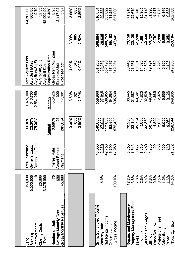
■
36
■
Cost and Revenue Assumptions
Financing Assumptions
Key Ratios
Rental Increase Projections
Average Monthly Rent
Operating Expense Projections
Operating Revenues
Operating Expenses
Actual Projected
Monthly Year 1 Year 2 Year 3 Year 4 Year 5
Table 3.4 Scenario I: 5 Year Pro Forma Income Statement As of January 1st
11532_Berges_c03.k.qxd 7/6/04 11:35 AM Page 36
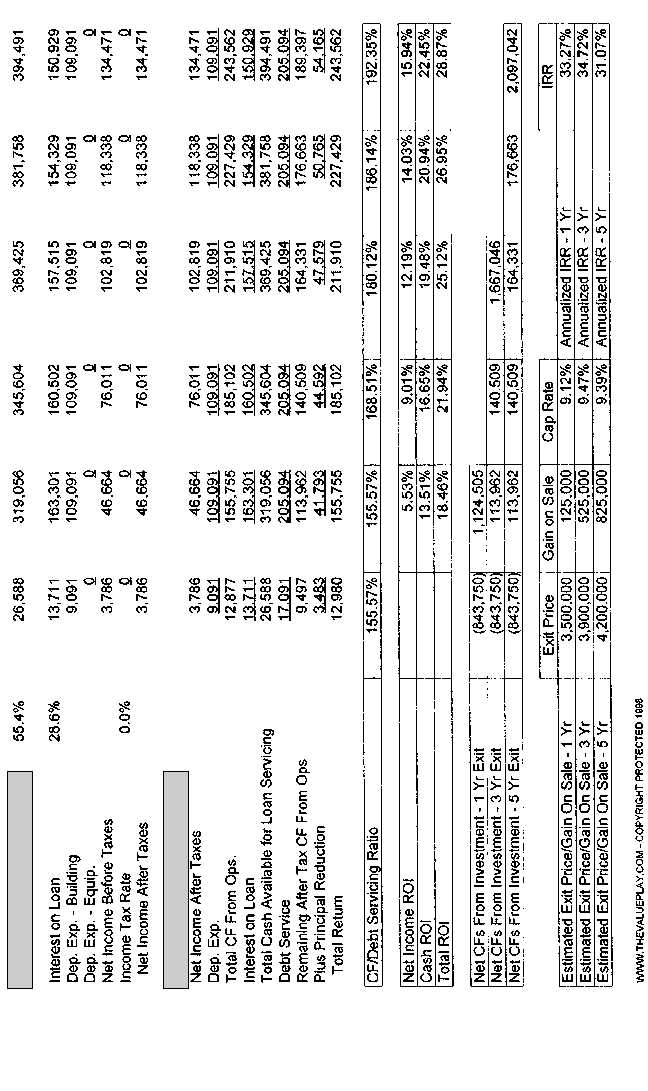
■
37
■
Net Operating Income
Cash Flow From Operations
11532_Berges_c03.k.qxd 7/6/04 11:35 AM Page 37
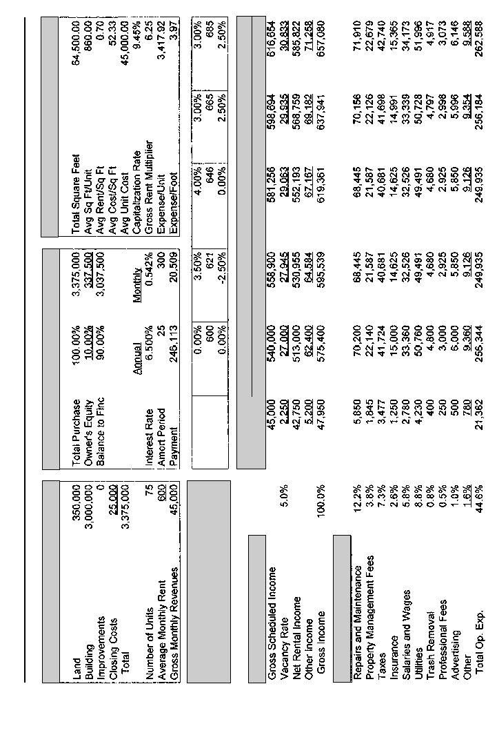
■
38
■
Cost and Revenue Assumptions
Financing Assumptions
Key Ratios
Rental Increase Projections
Average Monthly Rent
Operating Expense Projections
Operating Revenues
Operating Expenses
Actual Projected
Monthly Year 1 Year 2 Year 3 Year 4 Year 5
Table 3.5 Scenario II: 5 Year Pro Forma Income Statement As of January 1st
11532_Berges_c03.k.qxd 7/6/04 11:35 AM Page 38
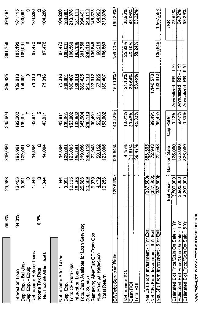
■
39
■
Net Operating Income
Cash Flow From Operations
11532_Berges_c03.k.qxd 7/6/04 11:35 AM Page 39

conversely, as the loan amount decreases, the down payment in-
creases. It is logical to assume that the more money borrowed, the
greater the monthly payment will be, and the less money borrowed,
the smaller the monthly payment will be. Although an investor
might conclude from this reasoning that it makes sense to put down
as much money as possible to decrease the monthly payment and
thereby increase the property’s cash flow, that conclusion would be
wrong. According to the other people’s money (OPM) principle,
which deals with the concept of leverage, the greater the percentage
of money borrowed the greater the return on equity will be. Even
though the monthly payment will increase by borrowing more, since
the returns are measured as a ratio of the income generated by the
property to the amount of one’s capital invested in it, the rate of
return is greater due to the increase in leverage. The OPM principle,
along with the principle of leverage, is discussed in greater detail in
the next chapter.
Several years ago, I developed a financial model I use extensively
to analyze and evaluate investment properties, which I call The
Value Play Income Analyzer. In Part 2, “Case Study Review, The
Practical Application of Valuation Analysis,” the model is explained
in much greater detail. For now, however, I’d like to focus on three
key measurements in the model. They are net income return on in-
vestment (net income ROI), cash ROI, and total ROI. Let’s take a
moment to examine the effect of changes in the amount of funds
borrowed on these three ratios by looking at two different scenarios.
In Table 3.4 (Scenario I), Investor A has used the Income Ana-
lyzer to evaluate an apartment building available for sale with a total
purchase price of $3,375,000. Under this scenario, the total amount
of funds borrowed by Investor A is $2,531,250. This leaves a bal-
ance of $843,750, or 25 percent, required for the down payment. In
this scenario, Investor A will realize a net income ROI of 5.53 per-
cent, a cash ROI of 13.51 percent, and a total ROI of 18.46 percent
in Year 1 on the invested capital, or cash down payment. Although
many investors would be satisfied with these returns, let’s see if
there is a way for us to improve them.
In Table 3.5 (Scenario II), all variables within the model are held
constant and are exactly the same as in Table 3.4 with the exception
■
Real Estate Finance for Investment Properties
■
■
40
■
11532_Berges_c03.k.qxd 7/6/04 11:35 AM Page 40

of two—the amount of funds borrowed and the down payment,
or owner’s equity. In Scenario II, the down payment has been
decreased to $337,500, which is a 10 percent investment, and the
amount of funds borrowed has been increased to $3,037,500. The
monthly payment required to service the debt in this scenario is
$20,509. This compares unfavorably to the monthly payment of
$17,091 in Scenario I and results in a net decrease of remaining after
tax cash flow (CF) of $3,418 per month.
At first glance, you may be inclined to believe that Investor A in
Scenario I is better off than Investor B in Scenario II, since Investor
A pockets an additional $3,418 per month. In Scenario II, Investor B
will realize a net income ROI of 4.15 percent, a cash ROI of 21.61
percent, and a total ROI of 36.47 percent in Year 1 on the invested
capital. According to our analysis, Investor B will earn almost twice
as much as Investor A. By increasing the amount of funds borrowed
and decreasing the amount of funds invested, you can actually earn
a higher rate of return on your invested capital. While it is true that
there is less cash remaining at the end of each period, the investor in
Scenario II fares much better than the investor in Scenario I. This is
because the returns are measured as a ratio of the remaining cash to
the investor’s equity or invested capital. Once again, by investing
less of your own money, you actually earn a higher rate of return
than you otherwise would, in spite of the fact that the remaining
cash has decreased.
In summary, the three secondary investment elements that affect
real estate financing activities are the cost of funds, the amortization
period, and the amount of funds borrowed. Understanding the inter-
action among these three variables and their relationship to one
another is essential for assessing how changes in any one of the
three can affect the profitability of the various types of real estate
investments. The better you understand these principles, the greater
will be your chances for success in the real estate business.
■
Secondary Investment Elements
■
■
41
■
11532_Berges_c03.k.qxd 7/6/04 11:35 AM Page 41

11532_Berges_c03.k.qxd 7/6/04 11:35 AM Page 42

Chapter 4
Additional Investment Elements
and Their Effect on
Financing Strategies
In Chapter 2, we examined the three primary financing elements
around which real estate investment activity centers—time, volume,
and property type. In Chapter 3 we learned about the three second-
ary financing elements that affect real estate financing activities—
cost of funds, amortization period, and amount of funds borrowed.
Three additional elements have an effect on real estate financing:
loan duration, lender fees, and prepayment penalties (see Exhibit
4.1). Duration must be considered before obtaining a loan to ensure
the life of it is best suited to an investor’s needs. It is also important
to be familiar with the many types of fees charged by lenders and to
know their effect on the overall cost of an investment. Finally,
investors should also be aware of any type of prepayment penalty
that may be imposed by the lender.
LOAN DURATION
The first additional element that has an effect on real estate financ-
ing is loan duration. Loan duration refers to a loan’s life, or term.
For instance, a loan duration of 10 years means that it will expire at
■
43
■
11532_Berges_c04.k.qxd 7/6/04 11:36 AM Page 43

the end of the 10-year period and must at its expiration either be
renewed or paid in full. A loan with a duration of 10 years may or
may not have an amortization period equal to its duration period.
Whereas amortization refers to the length of time used to calculate
the amount of payment to be made each period, duration refers to
the length of time the loan will exist. For example, a loan with a 10-
year duration, or term, can have a 15-, 20-, or 30-year amortization
period. At the end of its term, any remaining loan balance will have
to be repaid in full if the lender chooses not to renew or extend it.
Regardless of what type of financing is obtained for an investment
property, investors should be familiar with loan terms and the impact
they will have on their financing of real estate. Using the most appro-
priate term is best determined by the estimated length of time an
investment is intended to be held. For example, investors who intend
to hold a property for a period of 10 or more years would most likely
want to obtain a fixed-rate loan with a term that matches the full
amortization period, which is typically 30 years. Financing the prop-
erty with a shorter term, say five years, would force an investor to
refinance the property at the end of the term, or in five years.
Depending on the current interest rate environment, it may be bet-
ter to lock in a lower rate at the time of initial financing, since rates
can change suddenly and without notice. Investors who plan to hold
■
Real Estate Finance for Investment Properties
■
■
44
■
Exhibit 4.1
Additional financing elements.
1. Loan duration
2. Loan fees
3. Prepayment penalties
11532_Berges_c04.k.qxd 7/6/04 11:36 AM Page 44

a property for 10 years or more will need to procure a loan with a
corresponding time frame. If a decline in market interest rates
occurs at some point in the future, an investor always has the option
to refinance. If prepayment penalties exist, however, they, too, must
be factored into the refinance decision. An increase in market inter-
est rates will not affect the mortgage, because a measure of protec-
tion has been built in to insulate the investment from a higher-rate
environment by choosing the most appropriate financing term to
begin with.
Loans having longer durations can sometimes work to an in-
vestor’s disadvantage, especially if the property being purchased is
intended to be held for only a short while. If, for instance, a rehab
property has been identified and the property will be held for one
year or less before disposing of it, then a loan with a shorter duration
is preferable, because such loans typically have lower rates than
those with longer durations. This is because lenders can more accu-
rately predict interest rates over a shorter time frame than they can
over a longer time frame.
A one-year adjustable rate mortgage, or ARM, is almost certain to
have an interest rate ranging from
1
⁄2 to 1 percent lower than a loan
with a 30-year term. A one-year ARM typically has a fixed rate for
the first six months or one year, and then adjusts either annually or
semiannually thereafter. A comparable loan from a bank may carry
a rate to match a one-year ARM, but may also have a one-year term,
meaning that instead of adjusting, the loan will expire and have to be
satisfied by either renewing it or repaying it.
When selecting the duration or term that best meets an investor’s
financing needs, the investment objectives must first be determined.
Investors must establish beforehand how long a property is to be
held before committing themselves to a particular debt instrument.
Will the property be purchased and added to a portfolio containing
other rental properties and subsequently held for many years, or will
it instead be held for only a short period of time to capture a gain
created by making improvements to it? Investors should establish
their investment objectives prior to making a commitment to the
lender and then choose a loan with a duration best suited to the
desired opportunity.
■
Additional Investment Elements and Effect on Financing Strategies
■
■
45
■
11532_Berges_c04.k.qxd 7/6/04 11:36 AM Page 45

LOAN FEES
The second additional element that has an effect on real estate
financing is the loan fee assessed by the lender. Loan fees come in
all shapes and sizes and in all kinds of disguises. They are masked
by using terms such as application fees, review fees, underwriting
fees, loan-origination fees, mortgage broker fees, and points
charged at closing. Since some lenders are overly aggressive and
assess a fee or charge for just about everything, I suggest asking for
a list of all costs that will be charged by both the lender and the
mortgage broker (if applicable). Although by law lenders and bro-
kers are required to disclose all costs, these issues should be
addressed up front. Even after receiving the schedule of costs, it
pays to be careful, since some charges may show up on the settle-
ment statement at the last moment just prior to the loan closing. This
is especially true when using a mortgage broker.
Lenders are required by the federal Real Estate Settlement Proce-
dures Act to provide borrowers with a good faith estimate (GFE) of
the fees due at closing, and they must do so within three days of the
loan application. These mortgage fees, also called settlement costs,
cover the various expenses associated with mortgage financing.
Since closing costs usually range from between 3 and 5 percent of the
sale price, it’s best to wait until receiving a good faith estimate before
signing any loan. In fact, it’s a good idea to obtain good faith esti-
mates from several lenders and compare their respective costs. Take
just a moment to review the good faith estimate in Exhibit 4.2. The
form lists 15 different lender fees alone, as well as a number of addi-
tional fees by parties that may have an interest in the transaction.
Although the broker is legally obligated to disclose all reasonable
and customary fees, the broker doesn’t always know what fees the
lender will charge. The broker and the lender are not one and the
same. The broker acts as a third party to assist the purchaser in
obtaining the most appropriate type of financing. If brokers use
lenders they have not used before, they may not be aware of the
lender’s complete fee structure. I myself have been surprised on
more than one occasion by unexpected charges that show up at the
time of closing. I was especially surprised on a new build-to-suit
■
Real Estate Finance for Investment Properties
■
■
46
■
11532_Berges_c04.k.qxd 7/6/04 11:36 AM Page 46

■
47
■
Mailing Address Property Address
Proposed Loan Amount Estimated Interest Rate
Preparation Date
Loan Type
FHA VA Conventional Loan Number
The information provided below reflects estimates of the charges which you are likely to incur at the settlement of your loan. The fees
listed are estimates - actual charges may be more or less. Your transaction may not involve a fee for every item listed.
The numbers listed beside the estimates generally correspond to the numbered lines contained in the HUD-1 or HUD-1A
settlement statement which you will be receiving at settlement. The HUD-1 or HUD-1A settlement statement will show you
the actual cost for items paid at settlement.
"S"/ designates those costs to be paid by Seller/ . "A" designates those costs affecting APR.
These estimates are provided pursuant to the Real Estate Settlement Procedures Act of 1974, as amended (RESPA). Additional
information can be found in the HUD Special Information Booklet, which is to be provided to you by your mortgage broker or
lender, if your application is to purchase residential property and the Lender will take a first lien on the property.
HUD-1 DESCRIPTION OF CHARGES AMOUNT
GENESIS 2000, INC. * W14.0 * (800) 882-0504 Page 1 of 1 Form GFE (03/95)
This Good Faith Estimate is being provided by
a mortgage broker, and no lender has yet been obtained.
Broker"B" "F" designates financed costs.
Date Date
Date Date
801 Loan Origination Fee @ % + $
802 Loan Discount Fee @ % + $
803 Appraisal Fee
804 Credit Report
805 Inspection Fee
806 Mortgage Insurance Application Fee
807 Assumption Fee
808 Mortgage Broker Fee @ % + $
809 Tax Related Service Fee
810 Processing Fee
811 Underwriting Fee
812 Wire Transfer Fee
813 Application Fee
814 Commitment Fee
815 Lender's Rate Lock-In Fee
901 Interest @ /day for days
902 Mortgage Insurance Premium
903 Hazard Insurance Premium
904 County Property Taxes
906 Flood Insurance
1001 Hazard Ins. @ /mo. for months
1002 Mortgage Ins. @ /mo. for months
1004 Tax & Assmt. @ /mo. for months
1006 Flood Insurance @ /mo. for months
1008 Aggregate Escrow Adjustment
1101 Settlement or Closing/Escrow Fee
1102 Abstract or Title Search
1103 Title Examination
1105 Document Preparation Fee
1106 Notary Fee
1107 Attorney's Fee
1108 Title Insurance
1201 Recording Fee
1202 City/County Tax/Stamps
1203 State Tax/Stamps
1204 Intangible Tax
1301 Survey
1302 Pest Inspection
Exhibit 4.2 Good Faith Estimate
(not a loan commitment).
11532_Berges_c04.k.qxd 7/6/04 11:36 AM Page 47

home we sold several months ago that closed just recently. The
mortgage broker charged its client over $6,000 in broker fees for a
loan amount of only a little more than $200,000! That’s equivalent
to about 3 percent of the loan amount. What surprised me even
more, however, was that the homeowner had not even received a
good faith estimate until the day before the closing.
The loan application fee is a charge that some lenders assess at the
time formal application is made. Application fees range anywhere
from no charge at all to as much as $500 on single-family residential
properties. On larger commercial or multifamily loans, the initial
application fee can be as high as $2,500 to $5,000. The fee is charged
to offset costs incurred by the lender or broker for items such as
administrative costs and credit reports. Justification for the charges
results from a need to recover costs as well as the inability of some
applicants to qualify for loans. Charging an application fee serves to
filter out those individuals who may not be capable of qualifying for
a loan. If, for example, the applicant believes he may not be able to
qualify for a loan and knows an application fee of $250 will be
charged regardless of whether he qualifies, chances are he will not
bother with the application. Although lenders who charge an applica-
tion fee will most likely have fewer applicants, the quality of those
applicants is likely to be higher.
Application fees are oftentimes negotiable. If you know you have
good credit and will have no problem qualifying for a loan, be sure
to tell the lender or broker and ask for the application fee to be
waived. Many times the answer will be yes. The party taking the
application, however, may elect to charge the fee up front and agree
to credit it back to you at the time of closing. This helps reduce the
risk to the lender that the borrower will switch to another mortgage
company or bank at some point in the process. If the borrower has
paid a $500 application fee, for example, on a single-family invest-
ment property, or perhaps a $5,000 fee on a multifamily property,
and knows she will receive a credit for it at the time of closing,
there’s a very good chance she will stay with the lender to see the
loan through to the closing.
Underwriting fees have come about over the past few years as yet
another way to tack on additional charges. The justification for this
charge is similar to that of the application fee in that, similarly to
■
Real Estate Finance for Investment Properties
■
■
48
■
11532_Berges_c04.k.qxd 7/6/04 11:36 AM Page 48

personnel who are paid for processing the loan application, the
underwriting department must be paid for its job of underwriting the
loan. Using that logic, it seems reasonable to expect that at some
point in the future, we might begin seeing other types of fees show
up, such as a “loan committee fee” for reviewing the loan, or per-
haps a “human resources fee” to cover the cost of hiring all the other
departments that are charging us fees. The list is limited only by
one’s imagination.
Loan-origination fees, still another way of charging the borrower,
are usually equivalent to one point, or 1 percent, of the total amount
of the loan. On a $100,000 loan, for example, the fee would be
$1,000. Justification for this fee is supposedly based on the costs
incurred by the lender to actually make the loan once it has been
approved. Legal documents must be drawn up and processed, the
loan must be funded, and everything must be properly recorded.
Some lenders will waive the loan-origination fee altogether or roll it
into the interest rate on the loan by increasing the rate by 25 basis
points, which is the equivalent of one-fourth of a point.
Mortgage brokers earn the majority of their income from the fees
generated by placing loans. Since they are not direct lenders, bro-
kers do not earn anything from the interest being charged. Interest is
paid to the lender and not to the broker. A mortgage broker is simi-
lar to a real estate broker in that they are both compensated only
when they sell something. Both types of brokers are paid on a per-
centage basis. While the real estate agent is paid a commission, the
mortgage broker is paid points. Brokers typically charge between
1 and 2 percent of the loan amount, sometimes more and sometimes
less. Factors that may affect the fees they charge are items such as
the borrower’s creditworthiness, the size of the loan, and their abil-
ity to receive back-end fees from the lender. Don’t be fooled by bro-
kers who charge 1 percent on a $100,000 loan amount and tell you
they are making only $1,000 on the transaction. Brokers are almost
always compensated by the lender for differences in the spread of
the rate charged. For example, if the base rate a lender charges is
6.00 percent with zero points to the borrower, the broker will likely
be paid a back-end fee of 1 percent by the lender. If the broker is
able to sell the same loan to you at, let’s say 6.25 percent, the broker
can double his or her income on the loan and receive 2 percent from
■
Additional Investment Elements and Effect on Financing Strategies
■
■
49
■
11532_Berges_c04.k.qxd 7/6/04 11:36 AM Page 49

the lender. Both front-end and back-end fees are legally required to
be disclosed on the good faith estimate. Borrowers have a right to
know how much they are being charged for the lender’s services. If
you’re an investor with good credit and have a strong personal finan-
cial statement, mortgage brokers are less likely to play such games
with you. You’re probably familiar with the term caveat emptor, but
just in case you’re not, the literal translation means “buyer beware”
or “let the buyer beware.” In the case of loan fees, however, I sup-
pose we could say “let the borrower beware.”
Points are often made available to borrowers to buy down the
interest rate applied to a loan. Since one point is equivalent to 1 per-
cent, an investor paying one point on a $100,000 loan would pay
$1,000 in additional up-front fees. For every point paid, the interest
rate on the loan is decreased by approximately
1
⁄8 to
1
⁄4 of a percent.
This is only a general guideline, as rate spreads vary widely among
lenders, but the lender you are working with can usually provide an
exact quote by looking at rate sheets. Since rate spreads are dynamic
and change with minor fluctuations in the market, the rate quoted
may be good for just that particular moment, or it may be good for
the remainder of the day.
Take a moment to review Table 4.1. In this example, six different
rate scenarios are compared. The loan amount of $1 million and the
term of 240 months are held constant, while the interest rate and the
points are changed in each scenario. A base interest rate of 7.00 per-
cent with zero points is applied on the first line. In each subsequent
rate scenario, the interest rate is decreased in quarter-point increments
while simultaneously increasing the amount of discount points paid
by the borrower. In the first example, an investor who borrows $1 mil-
lion and pays no points and holds the loan throughout the duration of
its 20-year life would pay a total of $1,860,717.45, with a monthly
payment of $7,752.99. In the last example, the investor borrows the
same $1 million for the same 20-year period, but instead elects to
pay five discount points to buy the rate down from 7.00 percent to
5.75 percent. The investor in this scenario would pay a total of
$1,735,000.42, which includes the $50,000 for points paid, and would
have a monthly payment of $7,020.84. Buying down the rate in this
example would save the investor $732.15 per month and $125,717.03
■
Real Estate Finance for Investment Properties
■
■
50
■
11532_Berges_c04.k.qxd 7/6/04 11:36 AM Page 50
■
51
■
Table 4.1 Loan Comparisons
Symphony Homes, Inc. www.symphony-homes.com
The Value Play www.thevalueplay.com
Loan Amount Interest Rate Payments Points Payment Total Paid Cost of Loan Cost of Points
$1,000,000.00 0.07% 240 0% $7,752.99 $1,860,717.45 $860,717.45 $0.00
$1,000,000.00 0.0675% 240 1% $7,603.64 $1,834,873.62 $824,873.62 $10,000.00
$1,000,000.00 0.065% 240 2% $7,455.73 $1,809,375.53 $789,375.53 $20,000.00
$1,000,000.00 0.0625% 240 3% $7,309.28 $1,784,227.69 $754,227.69 $30,000.00
$1,000,000.00 0.06% 240 4% $7,164.31 $1,759,434.54 $719,434.54 $40,000.00
$1,000,000.00 0.0575% 240 5% $7,020.84 $1,735,000.42 $685,000.42 $50,000.00
Value Play Real Estate Software, 3.0.01 www.thevalueplay.com
11532_Berges_c04.k.qxd 7/6/04 11:36 AM Page 51

over the life of the loan. What this example assumes, however, is that
the investor will hold the property for the full twenty-year period. If an
investor determines ahead of time that a property is going to be main-
tained in her portfolio for the long term, then it makes sense to pay the
additional points up front. On the other hand, if the property is going
to be held for only five years, then it is better to pay the higher inter-
est rate with zero points. In this example, an investor would need to
hold the property for five years and nine months to realize any benefit
of paying the additional points. The break-even point can be calcu-
lated by dividing the cost of points over the savings per month. In this
example, the break-even point is calculated as follows:
Breakeven =
==68.29 months
One additional factor to consider is what the future value of the
$50,000 applied toward the discount points would be if it were
instead used to purchase another investment property. We have
already established that over a 20-year investment horizon, buying
the interest rate down by applying the $50,000 would save
$125,717.03 over and above all other costs. The question becomes,
can the $50,000 be used to invest in another asset over a 20-year
period to achieve an even greater return? To determine this, we must
solve for i, which is the rate required to earn a return on the invest-
ment of $125,717.03. To set the problem up correctly, we know that
$50,000 is the total amount invested, and $125,717.03 is the total
amount returned. Using a financial calculator, the answer can easily
be solved as follows:
Initial investment = present value = PV = $50,000 (cash flow out)
Total amount returned = future value = FV = $125,717.03 (cash
flow in)
Number of years = n = 20
$50,000
ᎏᎏᎏ
($7,752.99 − $7,020.84)
cost of points
ᎏᎏ
monthly savings
■
Real Estate Finance for Investment Properties
■
■
52
■
11532_Berges_c04.k.qxd 7/6/04 11:36 AM Page 52

To solve for the total return, solve for i
Interest rate = i = 4.72%
By solving for i, we discover that an investor would have to earn a
return of 4.72% or greater to come out ahead. If the investor could
not earn at least a 4.72% return, he would be better off paying down
the interest rate with the $50,000, assuming, of course, that the prop-
erty will be held for the 20-year duration.
Now let’s assume the investor has an alternative choice, which is
to invest the $50,000 in a small multifamily apartment building.
Let’s also keep the math very simple by assuming he is able to pur-
chase a building with only 10 percent down, which is not at all an
unreasonable assumption. Using this kind of leverage, the investor is
able to purchase a building valued at $500,000 ($50,000 ÷ 0.10 =
$500,000). Let’s also assume the investor purchased the property at
a 10 cap, which means the capitalization rate is 10 percent. An apart-
ment building with a cost of $500,000 and a cap rate of 10 will yield
a net operating income (NOI) of $50,000, which is the amount of
money left over after vacancy losses and operating expenses have
been deducted from gross revenues. It is the portion of income avail-
able to service, or pay, the debt used to finance an investment. Take
a moment to review the following equations.
Price ===$500,000
PV of apartment building == =$500,000
Cap rate ===10.0%
Now let’s take the analysis a step further by calculating the required
debt service on the $450,000 loan that was required to finance the
building. We’ll also assume the investor will use the same loan pro-
gram as he did with the first investment, as follows:
$50,000
ᎏ
$500,000
net operating income
ᎏᎏᎏ
price
$50,000
ᎏ
.10
NOI
ᎏ
cap rate
$50,000
ᎏ
0.10
net operating income
ᎏᎏᎏ
capitalization rate
■
Additional Investment Elements and Effect on Financing Strategies
■
■
53
■
11532_Berges_c04.k.qxd 7/6/04 11:36 AM Page 53

Loan amount = PV = $450,000
Number of years = n = 20
Interest rate = i = 7.0%
Annual debt service = pmt = $42,476.82
Let’s take a moment to recap. We have established that the invest-
ment of $50,000 in a $500,000 apartment building will yield $50,000
of NOI and will be used to pay the annual debt service of $42,476.82.
Where does that leave us? Let’s take a look.
$50,000.00 − $42,476.82 = $7,523.18 = remaining cash
= cash return on investment
$7,523.18/$50,000.00 = 15.05% cash ROI
In this example, the investor would earn a cash ROI of about 15
percent, which compares favorably to the 4.72 percent return if the
same $50,000 were used to buy down the interest rate. It is impor-
tant to note also that the cash ROI does not reflect the added value of
the tax savings resulting from depreciation, nor does it reflect the
added value of a reduction in the principal balance, or loan balance,
that occurs over the life of the loan. In summary, it appears that our
investor will fare much better by investing the $50,000 in an apart-
ment building than by buying down the interest rate on the purchase
of his first investment property.
PREPAYMENT PENALTIES
The third additional element that has an effect on real estate financ-
ing is known as a prepayment penalty. Although you would think a
bank or other lending institution would be happy to have its loan
repaid, believe it or not, many financial institutions charge their cus-
tomers a substantial fee for repaying a loan prematurely. This is
especially true on larger commercial and multifamily loans. You
may think, “Why would anyone want to pay off a loan early?” There
are two primary reasons loans are prepaid. The first is due to
changes in interest rates. If, for example, an investor obtained a large
■
Real Estate Finance for Investment Properties
■
■
54
■
11532_Berges_c04.k.qxd 7/6/04 11:36 AM Page 54

loan with a fixed rate of 7 percent, and rates then declined to 6 per-
cent, the investor would most likely want to take advantage of the
favorable change by refinancing. When people refinance, it is often-
times through another institution. This means the existing lender
loses a good loan to a competitor and, as a result, loses the income
associated with that loan. To discourage customers from refinancing
early in the life of the loan, lenders build in a prepayment penalty.
See Exhibit 4.3 for a sample of prepayment penalty disclosures.
The second primary reason loans are prepaid results from a
change in ownership. If, for example, an investor obtained a loan
with a five-year term that had a provision for a prepayment penalty
and decided to sell the property after just one year, the lender would
charge a fee, or penalty, for prepaying the loan. Up until the mid-
1980s or so, most loans were assumable, which meant the buyer
could assume, or transfer, the note into her name without having to
get a new loan. If the loan could be assumed by another party, then
it would not have to be prepaid and no penalty would be assessed.
Although assumable loans still exist, they are not nearly as common
as they used to be. In fact, most single-family mortgage notes have a
“due on sale” clause, which means that the note must be repaid in
full if a sale or transfer in ownership occurs.
Prepayment penalty fees are structured in numerous ways and can
sometimes be substantial. Prepayment fee structures range from a
simple declining penalty structure to a quite complex fee structure
for commercially oriented conduit loans. For example, a loan with a
simple declining prepayment penalty structure having a three-year
term may have a fee structure as follows:
Prepay Loan in Year Prepayment Penalty Fee
15%
24%
33%
40%
In this example, if an investor borrowed money and then decided to
repay the loan in Year 1, a penalty of 5 percent of the outstanding loan
balance would be imposed on her. If she repaid the loan in full in Year
■
Additional Investment Elements and Effect on Financing Strategies
■
■
55
■
11532_Berges_c04.k.qxd 7/6/04 11:36 AM Page 55

■
Real Estate Finance for Investment Properties
■
■
56
■
Exhibit 4.3
Prepayment penalty disclosure (2% penalty—Missouri).
YOU MAY HAVE TO PAY A PENALTY IF YOU SIGN A
PREPAYMENT PENALTY RIDER TO NOTE AND YOU
PREPAY ALL OR A PORTION OF YOUR LOAN AHEAD
OF SCHEDULE SET FORTH IN YOUR NOTE.
WHAT IS A PREPAYMENT?
“Prepay” means to pay more than your scheduled principal and
interest payment. Anything you pay in excess of your scheduled
monthly payment amount of principal and interest, provided you
have no outstanding late charges or other fees due, will be applied
to reduce, or prepay, your outstanding loan balance ahead of the
schedule contemplated in your Note. The most common form of
“prepayment” occurs when you payoff your loan in its entirety by
either refinancing or selling your property and using the sale pro-
ceeds to payoff the loan.
WHAT IS A PREPAYMENT PENALTY AND WHY SHOULD
I ACCEPT IT?
A prepayment penalty is a penalty you must pay if you prepay your
loan. It is your choice whether or not your loan has a prepayment
penalty. Generally speaking, your acceptance of a prepayment
penalty has value to your lender and to you. The lender benefits
because the risk of losing the investment in your loan is diminished
in the early years. You benefit because you are able to get a lower
interest rate and margin, and/or reduce your out-of-pocket closing
costs. In other words, if you want to waive the prepayment penalty,
your rate and margin may be higher, and/or your closing costs may
be increased. Ask us how your rate and margin and/or closing costs
would change without the Prepayment Penalty Rider to Note.
CAN YOU MAKE PREPAYMENTS WITHOUT PAYING A
PENALTY?
Yes. In any 12-month period during the term of the prepayment
penalty, you can prepay up to 20% of your original loan balance
11532_Berges_c04.k.qxd 7/6/04 11:36 AM Page 56

■
Additional Investment Elements and Effect on Financing Strategies
■
■
57
■
without penalty. After the term of the prepayment penalty, you can
prepay your loan without penalty.
DOES A PREPAYMENT PENALTY LAST FOR THE LIFE
OF THE LOAN?
No. The prepayment penalty applies only during the early term of
the loan. The most common “Prepayment Penalty Term is three
years, although your prepayment penalty term may be different (see
your prepayment penalty rider to note for your actual prepayment
penalty term). Once this term has expired, you will no longer have
to pay a prepayment penalty if you prepay your loan.
HOW IS THE PREPAYMENT PENALTY CALCULATED?
Your prepayment penalty is equal to 2 percent of the balance of the
Note. Any prepayment is payable at the time of the loan payoff or
upon request from the note holder.
PREPAYMENT PENALTY TERM
I have discussed my prepayment options with my loan officer and
have decided to obtain the following prepayment penalty term:
[ ] First five (5) years of the loan
Initials
[ ] First four (4) years of the loan
Initials
[ ] First three (3) years of the loan
Initials
[ ] First two (2) years of the loan
Initials
[ ] First one (1) year of the loan
Initials
[ ] No prepayment penalty
Initials
Acknowledged by:
_________________________ _________________________
Borrower Date Borrower Date
CS-004 09/99
Missouri
11532_Berges_c04.k.qxd 7/6/04 11:36 AM Page 57

2, she would incur a prepayment penalty of 4 percent of the remain-
ing loan balance. If the loan were repaid in Year 3, a 3 percent penalty
would be imposed. Finally, if she prepaid the loan at any time during
Year 4 or thereafter, there would be no prepayment penalty.
Let’s look at an example to determine how prepayment penalties
affect a loan transaction. In this example, Investor Green has just
acquired a small multifamily apartment building with a purchase
price of $800,000. While Investor Green has bought and sold many
single-family houses over the years, this transaction represents his
very first apartment deal. Since the loan amount is substantially
more than he is used to borrowing through his traditional financing
sources, Investor Green is forced to locate a new source of funding.
Investor Green is new to the world of high finance and agrees to a
loan with prepayment penalty fees structured as follows:
Prepay Loan in Year Prepayment Penalty Fee
14%
23%
30%
Investor Green closes on the property and is now the proud owner
of his first apartment building. Shortly after purchasing it, Green
happens to come across a book titled The Complete Guide to Buying
and Selling Apartments (New Jersey: John Wiley & Sons, 2004),
and discovers a technique that author Steve Berges refers to as the
value play. The value play strategy advocates a buy-and-sell philos-
ophy rather than a buy-and-hold approach. The idea is to purchase a
property that has upside potential, create value in it by making prop-
erty improvements, increasing revenues, and decreasing expenses,
and subsequently sell it to capture the gain, then move on to the next
deal and start the process over. Investor Green decides to implement
the value play strategy with his recent purchase and, after improving
the property and discovering ways to enhance its revenues, decides
to sell in Year 2. Let’s now take a look at how the prepayment penal-
ties affected his transaction. To keep the calculations simple, we’ll
also assume this is an interest-only loan with no payments made to
the principal balance.
■
Real Estate Finance for Investment Properties
■
■
58
■
11532_Berges_c04.k.qxd 7/6/04 11:36 AM Page 58

Purchase price = $800,000
Loan amount = $680,000
Interest rate = 6.25%
Loan origination Fee = 0.0%
Turnaround time = 18 months
Interest paid = $680,000 × 6.25% ÷ 12 × 18 = $63,750
Year 2 prepayment penalty = $680,000 × 3.0% = $20,400
Total interest and fees = $63,750 + $20,400 = $84,150
Effective interest rate = ($84,150 ÷ $680,000) ÷ 18 × 12 = 8.25%
As illustrated in this example, although the stated interest rate of
6.25 percent would be considered a competitive rate for most
investors, the effective rate of 8.25 percent is not nearly as attractive.
If our good friend Investor Green had been told up front that his
interest rate would be 8.25 percent, he probably would have politely
told the lender, “No thank you,” and moved on to the next lender.
Although he left an extra $20,400 on the table, because Green
adopted the value play strategy and applied it to this transaction, he
was able to walk away with a handsome profit. Next time around,
however, he’ll be a little wiser by negotiating with the lender in
advance for the best possible terms, which includes the elimination
of prepayment penalties.
As an investor, you should define your objectives with each and
every property you buy before you buy it. This includes defining your
time investment time horizon as well. If, for example, you intend to
purchase a property and implement the value play strategy, you know
you’re going to be holding the note for only a short period of time. If,
for instance, you obtained a $1 million loan with a 5 percent penalty
in Year 1 and prepaid it in that same year, you would be subject to
paying a penalty of $50,000. Ouch! No one wants to leave that much
money on the table. You can easily avoid getting into a situation like
this by knowing what your investment time horizon is ahead of time.
Understanding the nature of prepayment penalties and how they are
applied can potentially save you tens of thousands of dollars. Mini-
mize your exposure by obtaining a loan that doesn’t have a prepay-
ment penalty to begin with. Then you don’t have to worry about it.
In summary, three additional financing considerations investors
■
Additional Investment Elements and Effect on Financing Strategies
■
■
59
■
11532_Berges_c04.k.qxd 7/6/04 11:36 AM Page 59

need to be mindful of are a loan’s duration, any collateral fees that
may be charged by the lender or mortgage broker upon the origina-
tion of the loan, and any penalties which may be imposed as a result
of paying off the loan early. The prudent investor should obtain
financing with shorter durations to take advantage of more favorable
rates and also to lock in rates for longer durations for those invest-
ment opportunities that may have longer life cycles. The careful
investor should also use a cost-benefit analysis to determine whether
it makes sense to buy down the interest rate by paying additional
points up front. Finally, the careful investor will become familiar
with the specifics of any prepayment penalty clauses should they
exist.
■
Real Estate Finance for Investment Properties
■
■
60
■
11532_Berges_c04.k.qxd 7/6/04 11:36 AM Page 60

■
61
■
Chapter 5
Structuring Financial
Instruments
In Chapters 2, 3, and 4, we learned about the many different ele-
ments that directly impact financing for investment properties. Fac-
tors such as the time horizon, the volume of transactions, and the
type of property being purchased all influence an investor’s deci-
sion-making process. Furthermore, financing elements such as the
cost of funds, the amortization period, and the amount of funds
being borrowed affect the viability and profitability of a potential
investment opportunity. Finally, elements such as loan duration,
lender fees, and prepayment penalties will also have an impact on
whether an income-producing property can meet an investor’s return
criteria. In this chapter, we not only explore the different ways
investors can structure purchases, but also the advantages and disad-
vantages of each (see Exhibit 5.1). We also analyze the effect these
various financing mechanisms have on returns.
LEVERAGE
A lever is a tool supported by a fulcrum that can be used to lift heavy
objects. Archimedes, an ancient Greek mathematician and physicist,
calculated the law of the lever. He is reported to have said that if he
had a lever long enough and a fulcrum large enough, he could lift the
world. When applied to real estate, the principle of leverage enables
11532_Berges_c05.k.qxd 7/6/04 11:36 AM Page 61

investors to purchase properties they would otherwise not be capa-
ble of purchasing. Applying the law of leverage to the various
financing mechanisms that are available can potentially allow indi-
viduals to greatly magnify the return on their investments. In fact,
without leverage, many people would not even be able to purchase
real estate since they can barely save enough money to make even a
small down payment.
Investors use the law of leverage to help them lever up the returns
on their holdings. The application of this law suggests that investors
will use a lever to lift something that they would otherwise not be
able to lift. The lever is supported by a fulcrum, which is defined as
the support on which the lever turns. In the case of real estate, the
fulcrum represents the use of other people’s money, commonly
referred to as the OPM principle. On one end of the lever is an
investor’s initial capital outlay, however small it may be, and on the
other end of the lever is the real estate being levered. The fulcrum
enables investors to apply the law of leverage.
The law of leverage as it applies to real estate rests on the prem-
ise that the cost of other people’s money must be less than the return
■
Real Estate Finance for Investment Properties
■
■
62
■
Exhibit 5.1
Structural elements.
1. Leverage
2. Debt
3. Equity
4. Partnerships
5. Blended financing and WACC
6. Options
11532_Berges_c05.k.qxd 7/6/04 11:36 AM Page 62

on the asset being invested in. For example, if an investor borrows
funds from a financial institution in the form of debt, the cost of that
debt must be less than the expected return on the assets it is invested
in. If it is not, then it makes no sense to borrow those funds, because
the investor will lose money.
Let’s look at a simple example. If the interest rate on a loan is
6.0 percent and the expected return on assets (ROA) is 10 percent,
then the leverage is said to be positive and would represent a viable
investment opportunity. On the other hand, if the cost of funds is
8.5 percent and the expected ROA is 5.75 percent, the leverage is
said to be negative and would not represent a viable investment
opportunity. The difference between the cost of funds and the ROA
is referred to as the spread. One of the most common mistakes
novice investors make is based on the false assumption that any
property purchased with nothing down must be a good investment
since they didn’t have to put any money down. What they fail to real-
ize, however, is that if the property has a negative spread and a neg-
ative monthly cash flow because it is highly leveraged, the
investment will not generate a positive return. On the contrary, it
will generate a negative return requiring monthly cash injections
that can literally destroy investors if they have no reserves.
Take a moment to review Table 5.1. It illustrates the effect of price
appreciation using no leverage and an initial investment of
$500,000, which represents 100 percent of the purchase price. The
table applies 5, 10, and 20 percent growth rates over a period of
25 years. An investor in this scenario using an annual growth rate
of 5 percent will enjoy a total return of 238.6 percent over the
25-year period. Not bad.
Now let’s compare the returns in Table 5.1 to those in Table 5.2,
which illustrates the effect of price appreciation on leverage using
an initial investment of $75,000, or 15 percent of the purchase price.
This table also applies 5, 10, and 20 percent growth rates over a
period of 25 years. An investor in this scenario using an annual
growth rate of 5 percent will enjoy a total return of a remarkable
1,590.9 percent over the same 25-year period! The use of leverage
has allowed the investor in the second scenario to enjoy a return
almost seven times greater than the investor in the first scenario.
■
Structuring Financial Instruments
■
■
63
■
11532_Berges_c05.k.qxd 7/6/04 11:36 AM Page 63

Table 5.1 Effect of Leverage on Invested Capital Applying Annual
Appreciation Only
Purchase Price: $500,000
Percent Down: 100.0%
Down Payment: $500,000
Number
Annual Appreciation Rate
of Years 5.0% Ret on Inv 10.0% Ret on Inv 20.0% Ret on Inv
1 525,000 5.0% 550,000 10.0% 600,000 20.0%
2 551,250 10.3% 605,000 21.0% 720,000 44.0%
3 578,813 15.8% 665,500 33.1% 864,000 72.8%
4 607,753 21.6% 732,050 46.4% 1,036,800 107.4%
5 638,141 27.6% 805,255 61.1% 1,244,160 148.8%
6 670,048 34.0% 885,781 77.2% 1,492,992 198.6%
7 703,550 40.7% 974,359 94.9% 1,791,590 258.3%
8 738,728 47.7% 1,071,794 114.4% 2,149,908 330.0%
9 775,664 55.1% 1,178,974 135.8% 2,579,890 416.0%
10 814,447 62.9% 1,296,871 159.4% 3,095,868 519.2%
11 855,170 71.0% 1,426,558 185.3% 3,715,042 643.0%
12 897,928 79.6% 1,569,214 213.8% 4,458,050 791.6%
13 942,825 88.6% 1,726,136 245.2% 5,349,660 969.9%
14 989,966 98.0% 1,898,749 279.7% 6,419,592 1183.9%
15 1,039,464 107.9% 2,088,624 317.7% 7,703,511 1440.7%
16 1,091,437 118.3% 2,297,486 359.5% 9,244,213 1748.8%
17 1,146,009 129.2% 2,527,235 405.4% 11,093,056 2118.6%
18 1,203,310 140.7% 2,779,959 456.0% 13,311,667 2562.3%
19 1,263,475 152.7% 3,057,955 511.6% 15,974,000 3094.8%
20 1,326,649 165.3% 3,363,750 572.7% 19,168,800 3733.8%
21 1,392,981 178.6% 3,700,125 640.0% 23,002,560 4500.5%
22 1,462,630 192.5% 4,070,137 714.0% 27,603,072 5420.6%
23 1,535,762 207.2% 4,477,151 795.4% 33,123,686 6524.7%
24 1,612,550 222.5% 4,924,866 885.0% 39,748,424 7849.7%
25 1,693,177 238.6% 5,417,353 983.5% 47,698,108 9439.6%
This simple example does not even take into consideration the effect
of income generated, tax benefits, or principal reduction.
DEBT
In The Complete Guide to Investing in Rental Properties (New York:
McGraw-Hill, 2004), I described the use of debt in the following
excerpt.
■
Real Estate Finance for Investment Properties
■
■
64
■
11532_Berges_c05.k.qxd 7/6/04 11:36 AM Page 64

Other people’s money can be provided to you in one of
two forms—either debt or equity. The most common type
of financing is debt. Debt is most often provided in the
form of some type of loan which can come from any num-
ber of sources including banks, mortgage companies, fam-
ily members, friends, credit cards, and home equity loans
to name a few. Financing with debt typically requires that
you repay a loan with predetermined terms and conditions
such as the repayment term (number of years to repay the
■
Structuring Financial Instruments
■
■
65
■
Table 5.2 Effect of Leverage on Invested Capital Applying Annual
Appreciation Only
Purchase Price: $500,000
Percent Down: 15.0%
Down Payment: $75,000
Number
Annual Appreciation Rate
of Years 5.0% Ret on Inv 10.0% Ret on Inv 20.0% Ret on Inv
1 525,000 33.3% 550,000 66.7% 600,000 133.3%
2 551,250 68.3% 605,000 140.0% 720,000 293.3%
3 578,813 105.1% 665,500 220.7% 864,000 485.3%
4 607,753 143.7% 732,050 309.4% 1,036,800 715.7%
5 638,141 184.2% 805,255 407.0% 1,244,160 992.2%
6 670,048 226.7% 885,781 514.4% 1,492,992 1324.0%
7 703,550 271.4% 974,359 632.5% 1,791,590 1722.1%
8 738,728 318.3% 1,071,794 762.4% 2,149,908 2199.9%
9 775,664 367.6% 1,178,974 905.3% 2,579,890 2773.2%
10 814,447 419.3% 1,296,871 1062.5% 3,095,868 3461.2%
11 855,170 473.6% 1,426,558 1235.4% 3,715,042 4286.7%
12 897,928 530.6% 1,569,214 1425.6% 4,458,050 5277.4%
13 942,825 590.4% 1,726,136 1634.8% 5,349,660 6466.2%
14 989,966 653.3% 1,898,749 1865.0% 6,419,592 7892.8%
15 1,039,464 719.3% 2,088,624 2118.2% 7,703,511 9604.7%
16 1,091,437 788.6% 2,297,486 2396.6% 9,244,213 11659.0%
17 1,146,009 861.3% 2,527,235 2703.0% 11,093,056 14124.1%
18 1,203,310 937.7% 2,779,959 3039.9% 13,311,667 17082.2%
19 1,263,475 1018.0% 3,057,955 3410.6% 15,974,000 20632.0%
20 1,326,649 1102.2% 3,363,750 3818.3% 19,168,800 24891.7%
21 1,392,981 1190.6% 3,700,125 4266.8% 23,002,560 30003.4%
22 1,462,630 1283.5% 4,070,137 4760.2% 27,603,072 36137.4%
23 1,535,762 1381.0% 4,477,151 5302.9% 33,123,686 43498.2%
24 1,612,550 1483.4% 4,924,866 5899.8% 39,748,424 52331.2%
25 1,693,177 1590.9% 5,417,353 6556.5% 47,698,108 62930.8%
11532_Berges_c05.k.qxd 7/6/04 11:36 AM Page 65

loan), the interest rate, and any prepayment penalties
which may be imposed for paying off a loan early.
One primary advantage of using debt is its lower cost of
capital than other forms of financing such as equity. Another
advantage of using debt is that it is typically more readily
available than equity. One key disadvantage of using debt is
that the debt must be serviced. In other words, you have to
make periodic payments on the loan. Using debt as a source
of financing will usually have a direct negative impact on
the cash flow from your rental house since loans usually
require monthly payments. It should be obvious to you that
the more you borrow for a particular investment, the greater
your monthly payment will be, and the greater your monthly
payment, the less the property’s after tax cash flow will be.
As a smart investor, you must be sure that you have struc-
tured the purchase of your rental house in such a manner
that will allow you to service the debt on it, whatever the
source of that debt is, without a negative cash flow. This is
after all expenses have been accounted for. You should have
a minimum of a 1.1 to 1.2 ratio of free cash flow left over
after all expenses have been paid to ensure that you can
adequately meet the debt requirements. Debt is a wonderful
tool, but like any tool, you must exercise caution and
respect when using it. Otherwise you can quickly find your-
self in trouble. You must be in control of your debt. Do not
allow your debt to control you.
From this excerpt, we learn that the primary advantages of using
debt are that it is readily available and that it can typically be
obtained at a lower cost than alternative financing sources such as
equity. In Chapter 3, we examined the effect of different interest
rates on the value and returns of an income-producing property. The
lower the cost of funds, the greater the cash flow, and the greater the
cash flow, the greater an investor’s returns.
We also learned that one key disadvantage is that debt usually
requires that some type of periodic payment be made. This is espe-
cially important because an investor purchasing a non-income-
producing property may have a difficult time making the required
■
Real Estate Finance for Investment Properties
■
■
66
■
11532_Berges_c05.k.qxd 7/6/04 11:36 AM Page 66

periodic payments. For example, when I purchase land on which to
build houses, my preference is to defer all interest and tax pay-
ments for as long as I can. If possible, I structure the financing in
such a manner that no payments are due until a lot is released.
When a house is ready to be built on a particular lot, all accrued
interest and taxes are paid on the lot at that time. The payment is
made from the construction loan used to build the house. Structur-
ing the financing in this manner enables me to lever up without
having the burden of making periodic payments on the land.
One additional advantage of using debt is that the interest portion of
the payment is tax deductible, because interest is treated as an expense
for tax purposes. Since the interest portion of a debt payment is tax
deductible, the effective interest rate is lower than it otherwise would
be. This provides investors with an added incentive to use debt rather
than equity, since they are able to further reduce their cost of funds.
Let’s take a moment to look at an example to see how this works.
Loan amount = $100,000
Interest rate = 6.50%
Annual interest paid = $100,000 × 6.50% = $6,500
Investor’s tax rate = 35%
Reduction in taxes = $6,500 × 35% = $2,275
Effective interest rate = ($6,500 − $2,275) = $4,225 ÷ $100,000
= 4.225%
This example assumes a loan amount of $100,000 and cost of funds
of 6.50 percent. An investor in a 35 percent tax bracket would real-
ize $2,275 in savings as a result of the reduction in tax liability. The
annual cost of funds is reduced from $6,500 to $4,225, which in turn
reduces the effective tax rate to 4.225 percent.
EQUITY
Another common method of funding an investment is by raising
capital in the form of equity. Whereas debt represents money that is
borrowed, equity represents money that is invested. Equity financ-
ing can be provided by any number of sources and commonly
■
Structuring Financial Instruments
■
■
67
■
11532_Berges_c05.k.qxd 7/6/04 11:36 AM Page 67

involves the formation of a legal partnership or corporation. Family,
friends, business associates, and private investors can all be good
sources of equity financing. One of the main reasons for using
equity financing is to minimize the cash flowing out of income-
producing properties. The repayment of equity financing can be
structured in any number of ways. For example, you can agree with
the investor to pay a specified percentage of the profits at the end of
each quarter, semiannually, or even annually. You could also agree to
defer all payments until such time as the property is sold. Sharing
profits with an equity investor can be based on income, capital
gains, or any combination of the two. Preserving as much cash as
possible, especially in the earlier years of investing when cash
reserves tend to be smaller, can mean the difference between success
and failure in the real estate business.
Although not as common as lenders who provide financing in the
form of loans, or debt, a number of institutional investors are willing
to fund investment projects in the form of equity. In other words,
instead of lending money to buyers, investors contribute capital in
the form of equity. In essence, they become shareholders. Capital
contributions from equity investors allow the smaller private
investors to leverage up into larger commercial or multifamily prop-
erties that they otherwise would not be capable of purchasing.
Equity investors typically require a minimum return on their
investment that is higher than if the funds had been borrowed. Fur-
thermore, because they are shareholders, equity investors also
expect to share in the profits of a property that result from its sale.
Most of the larger institutional investors are looking to place large
sums of capital and oftentimes will not even consider a project less
than $5 million in size. Since they will fund up to 80 or 90 percent
of the capital required, the private investor will need to be prepared
to invest a minimum of 10 to 20 percent. Let’s look at an example to
see how this might work for a commercial strip center with a pur-
chase price of $5 million.
Purchase price = $5,000,000
Total equity = 20% = $5,000,000 × 20% = $1,000,000
Institutional share = 80% = $1,000,000 × 80% = $800,000
Investor share = 20% = $1,000,000 × 20% = $200,000
■
Real Estate Finance for Investment Properties
■
■
68
■
11532_Berges_c05.k.qxd 7/6/04 11:36 AM Page 68

Structuring the financing in this manner allows smaller investors
the opportunity to acquire larger income-producing properties than
would otherwise be possible. In this example, the investor is able to
purchase a $5 million commercial property with only $200,000.
Instead of the normal 15 to 20 percent down, the investor has to
come up with only 4 percent of the total purchase price, as follows:
Investor share of total purchase price ==4%
Institutional firms like partnering with local investors who are
familiar with the market in a specific area. Local investors often-
times have a good idea of which areas are preferable for various rea-
sons. For example, they may have insight into which areas are
enjoying positive, even strong, growth and which areas are deterio-
rating and should likely be avoided. Local investors can also help
with, or even be responsible for, the management of the property.
Don’t assume that institutional firms are standing by with an open
checkbook waiting to invest in the first property that you bring to
them. That isn’t the case. These investors have accumulated large
pools of capital because they are very careful, not because they throw
money at every opportunity presented to them. As a smaller investor
who is familiar with the local market, you will have to carefully select
a property that you believe has potential and represents a sound invest-
ment. Then you need to be prepared to put together a well-thought-out
business plan, which will include data specific to the area and the
property, such as the unemployment rate, average vacancy rates, and
rental rates for similar properties. Institutional investors are very
selective when they purchase properties, so be prepared to sell them
not only on the property and the area, but on yourself as well.
PARTNERSHIPS
Combining your own resources with those of a partner is another
way to raise financing for investment properties. The type of partner
I am referring to in this section is a friend, family member, or busi-
ness acquaintance. This differs from the large institutional investor
$200,000
ᎏᎏ
$5,000,000
■
Structuring Financial Instruments
■
■
69
■
11532_Berges_c05.k.qxd 7/6/04 11:36 AM Page 69

described in the previous equity financing section. Partnerships can
be structured in a variety of ways. For instance, capital infusions by
partners can take the form of debt or equity, partners can play an
active or a passive role, and terms for the repayment provisions can
be defined in any number of creative ways. While bringing in a part-
ner certainly has its advantages, probably one of the most challeng-
ing aspects is finding one you can work with.
If your partner participates simply by loaning money in the form
of debt, then a fixed amount will be repaid to that partner under pre-
defined terms and conditions. Unlike more traditional sources of debt
financing, payments can be structured in any manner the two of you
agree on. For example, you may agree to make both principal and
interest payments, interest-only payments, or perhaps defer all pay-
ments until the property is sold. Regardless of how the payments are
structured, the amount repaid is predetermined as set forth in a fully
executed promissory note and is not based on the profitability of the
property. Furthermore, the two of you may choose to secure the loan
by the property, or you may choose to secure it by some other form
of collateral, or you may choose not to secure the loan at all. At a
minimum, the promissory note should be witnessed and recordable.
The two of you may choose not to record the note for any number of
reasons, but the partner loaning the money should have the right to
record the instrument if he or she so chooses. An alternative to secur-
ing debt financing from a partner is to obtain equity financing. If your
partner agrees to invest in your project using equity, then he or she
will share the risk with you. If your project goes south, your partner’s
investment in the project goes south with you. On the other hand, if
you hit a home run, your partner will score right along with you. Both
you and your partner will enjoy the benefit of sharing in the profits.
Partners may take either an active or passive role in helping you
manage and operate the property. For example, you may decide to
have your partners actively participate by taking advantage of what-
ever skill sets they may have. If they have good management skills,
for instance, you may want them to help manage the property. On the
other hand, you may choose to have your partners play a completely
passive role wherein their only contribution is investment capital. In
summary, allowing partners to participate can be beneficial to you by
■
Real Estate Finance for Investment Properties
■
■
70
■
11532_Berges_c05.k.qxd 7/6/04 11:36 AM Page 70

providing additional capital for a project that otherwise may be out of
reach financially. Finally, partners may be able to contribute services
or specific skills that you may be lacking.
We’ve discussed several of the advantages of working with part-
ners. Now let’s take a moment to review some of the challenges.
Perhaps the biggest of them is finding the right partner to work with.
Just as a married couple who are in tune with each other can live and
work and dream together in harmony year after year, so can partners
work together to achieve great financial success. As in a marriage,
success requires give and take in the relationship. The partners must
be able to get along with each other and work together in a spirit of
harmony. There must always be a cooperative effort exerted by each
partner. This doesn’t mean there can’t be any disagreements, for cer-
tainly there will be; however, you need to have the ability to resolve
your differences peaceably.
It also helps to clearly define each partner’s duties and responsi-
bilities and to then allow them to work within the agreed-upon
framework. As with our spouses, we are sometimes too quick to crit-
icize and too slow to compliment. It is tempting to micromanage
other people’s performance and point out that they are “not doing it
the right way.” Working closely together with a partner takes just the
right balance of temperament and respect for each other. Husbands
and wives often search for years to find the right companion; even
then, marriages often result in divorce. Finding the right partner to
work with does not happen overnight. Even when you think you
may have found the right business partner, the relationship can fail
for any number of reasons.
You should consider in advance before ever forming a partnership
how its potential failure may affect the relationship you have with that
individual, especially if it is a family member. I know of one particu-
lar instance where a father-in-law invested much of his savings in his
son-in-law’s residential construction business. Two years later, the
family business went belly-up when the son-in-law declared bank-
ruptcy. I’m sure this failure placed a tremendous strain on the family’s
relationships. On a more successful note, however, I am equal partners
with my brother-in-law, Don Mahoney, in our residential construction
company, Symphony Homes. I respect his role as the master builder
■
Structuring Financial Instruments
■
■
71
■
11532_Berges_c05.k.qxd 7/6/04 11:36 AM Page 71

of our homes, and he in turn respects my role as the master builder of
our company. I don’t try to tell him how to build the houses, and he
doesn’t try to tell me how to build the company. That’s not to say that
we don’t have input for each other. He offers his comments and opin-
ions to me, which I gratefully accept, and I offer my comments and
opinions to him. Although we have our differences from time to time,
it has definitely been a win-win partnership for us. Without Don to
ensure that each and every home is built as it should be, I would not
have been able to enjoy a fraction of the success in our company that
I do today. Likewise, without me to develop our business, Don
wouldn’t have nearly as many houses to build as he does today.
BLENDED FINANCING AND THE
WEIGHTED AVERAGE COST OF CAPITAL
When purchasing income-producing properties, especially larger
ones, investors often combine several sources of financing, including
both debt and equity. For example, an investor may purchase a 450-
unit apartment building using a first mortgage for 70 percent of the
total purchase price plus improvements, then raising another 15 per-
cent of the total purchase price plus improvements through equity
arrangements, then borrowing an additional 10 percent of the total
for capital improvements from another lender, and finally, investing
5 percent of his or her own capital. Since the four different sources
that provide the financing will most likely charge different rates, a
blended rate must be calculated. This blended rate is known as the
weighted average cost of capital (WACC). A company’s WACC is
the average rate of return required by all of its creditors and investors.
Calculating the WACC for a business or company enables its own-
ers to determine the threshold for future projects or investments. If a
real estate firm holding a portfolio of properties, for instance, calcu-
lated its WACC at 7.40 percent, assuming the firm’s cost of capital
was held constant, it would have to be able to earn a minimum of
7.40 percent to justify investing in another property. If the expected
return was less than 7.40 percent, the firm would retain its investment
resources until a more favorable opportunity presented itself.
■
Real Estate Finance for Investment Properties
■
■
72
■
11532_Berges_c05.k.qxd 7/6/04 11:36 AM Page 72

An investment firm’s cost of capital is calculated by first deter-
mining the weight of each component of debt or equity and then
multiplying that weight by its respective cost. Take a moment to
study the following formula.
Weighted average cost of capital = (proportion of debt × cost of
debt) + (proportion of equity × cost of equity) = WAC C
The formula can also be written as follows:
Weighted average cost of capital =
冢冣
× bond rate +
冢冣
× securities rate = WAC C
WAC C =
冢冣
× R
B
+
冢冣
× R
S
where
WACC is the firm’s weighted average cost of capital
B is the value of bonds, or debt, used for financing
S is the value of stocks, or equity, used for financing
R
B
is the cost of debt, or interest rate
R
S
is the cost of equity, or the expected return on equity
Now let’s apply the WACC formula to an example. Assume the fol-
lowing:
Value of real estate portfolio = $25 million
Total outstanding debt = $20 million
Total outstanding equity = $5 million
Average cost of debt = 6.20%
Average cost of equity = 10.40%
S
ᎏ
B + S
B
ᎏ
B + S
securities
ᎏᎏ
bonds + securities
bonds
ᎏᎏ
bonds + securities
■
Structuring Financial Instruments
■
■
73
■
11532_Berges_c05.k.qxd 7/6/04 11:36 AM Page 73

WAC C =
冢冣
× 6.20%
+
冢冣
× 10.40% =
冢冣
× 6.20% +
冢冣
× 10.40% = (.80 × .0620)
+ (.20 × .1040) = .0496 + .0208 = .0704 = 7.04% = WAC C
In this example, the weighted average cost of capital for the real
estate portfolio is 7.04 percent. If the investment firm that owned the
portfolio decided to purchase another property, its managers would
carefully examine the firm’s cost structure. Assuming a similar cost
structure was required to purchase the property, then the manager’s
threshold would be a minimum of 7.04 percent. That means the total
return from the property must yield an income stream of at least 7.04
percent to increase the total return to the firm. Anything less than
that means that the cost of financing the property would be greater
than the income earned from it and would therefore have a negative
impact on earnings.
Although the WACC calculation is a useful tool for individuals or
businesses investing on a larger scale, it is just as useful for those
individuals or businesses investing on a smaller scale. As an exam-
ple, an investor buying a $1 million commercial building must pull
$200,000 out of her mutual fund, which has been averaging a 12.0
percent rate of return. She will borrow the remaining $800,000 at an
interest rate of 6.0 percent. The WACC in this example would be as
follows:
WAC C =
冢冣
× 6.00%
+
冢冣
× 12.00% =
冢冣
$800,000
ᎏᎏ
$1,000,000
$200,000
ᎏᎏᎏ
$800,000 + $200,000
$800,000
ᎏᎏᎏ
$800,000 + $200,000
$5,000,000
ᎏᎏ
$25,000,000
$20,000,000
ᎏᎏ
$25,000,000
$5,000,000
ᎏᎏᎏ
$20,000,000 + $5,000,000
$20,000,000
ᎏᎏᎏ
$20,000,000 + $5,000,000
■
Real Estate Finance for Investment Properties
■
■
74
■
11532_Berges_c05.k.qxd 7/6/04 11:36 AM Page 74

× 6.00% +
冢冣
× 12.00% = (.80 × .0600)
+ (.20 × .1200) = .0480 + .0240 = .0720 = 7.20% = WAC C
At first glance, it appears that because the WACC is 7.20 percent,
our investor is better off leaving her money in the mutual fund so it
can continue to earn 12.00 percent rather the 7.20 percent shown in
the calculation; however, because financial leverage was introduced,
this may or may not be the case. If the property was purchased at a
capitalization rate of 8.50 percent, that means its net operating
income would be $85,000 annually before interest. Applying a sim-
ple interest-only calculation would require annual debt service as
follows:
Net operating income = $85,000
Debt service = $800,000 × 6.00% = $48,000
Net income before taxes = $37,000
Now let’s compare the earnings of $37,000 to the yield on our
investor’s savings if left in her mutual fund.
Mutual fund savings = $200,000
Expected rate of return = 12.00%
Earnings before taxes = $24,000
Difference between investments = $37,000 − $24,000 = $13,000
Yield on investor’s equity = $37,000/$200,000 = 18.50%
In this simple example, by introducing the concept of financial
leverage, the investor would be able to earn an 18.50 percent rate of
return by purchasing the commercial building versus a 12.00 per-
cent rate of return by leaving her money invested in a mutual fund.
Calculating the weighted average cost of capital enables the investor
to better understand her true cost of capital. Although she is borrow-
ing funds at an interest rate of 6.00 percent, because she is investing
funds that would otherwise earn 12.00 percent, her true WACC is
7.20 percent.
$200,000
ᎏᎏ
$1,000,000
■
Structuring Financial Instruments
■
■
75
■
11532_Berges_c05.k.qxd 7/6/04 11:36 AM Page 75

OPTIONS
Option agreements are used by investors to gain control of an asset
without having to take legal title to it. Options give investors the
legal right to purchase an asset at a predetermined price. The use of
options is used by investors every day in the stock market to gain
control of the rights to either buy or sell various types of securities.
An investor could purchase, for instance, a put option for 1,000
shares of Intel with a strike price of $35. This gives the investor the
right to sell shares of Intel at $35. The Black-Scholes model is the
standard by which options are valued. As with all options, time t is
one of the variables that determine its value. Investors have the
right to exercise an option at their discretion within a specified
period of time. While it is possible that an investor will buy or sell
at precisely the right time to lock in a gain, it is also possible that
the option will expire worthless and that the investor will lose the
money invested to purchase it. In the case of the investor who pur-
chased a put option for 1,000 shares of Intel, it is hoped that the
price of the stock will fall so that the investor can sell it at the
higher strike price of $35 after having purchased it at any price less
than its strike price.
An option works essentially the same way with real estate as it
does with a stock. Some sellers may require the purchaser to meet
additional obligations, such as assuming responsibility for interest
and taxes; however, these items are negotiable. When an option is
used with real estate, investors have the legal right to purchase a
specified piece of property at a predetermined price within a given
time frame. As with stocks, t will eventually expire worthless if the
option is not exercised. At some point before the expiration of the
option agreement, the investor may exercise her right to purchase
the property at whatever price was established. In addition, since a
legal interest is held in the property, that interest is usually trans-
ferable. This gives the investor the right to sell the property with-
out ever taking title to it. Options are a terrific tool investors can
use to purchase property with very little cash of their own. This is
especially true if another buyer is found before actually having to
take title to it. Another benefit of using options is that they provide
■
Real Estate Finance for Investment Properties
■
■
76
■
11532_Berges_c05.k.qxd 7/6/04 11:36 AM Page 76

investors with the ability to limit their risk exposure in a particular
property to only the premium paid for the option. If the investor
decides not to exercise the right to purchase, the option expires
worthless, and only the premium paid for the option is lost.
Depending on the value of the subject property, an option may
potentially cost tens of thousands of dollars. While this may repre-
sent a substantial amount of money, keep in mind that the price
paid for an option is relative to the value of the property being
sought. Although the Black-Scholes model is the standard used to
price options for stocks, option premiums for real estate are typi-
cally based on whatever price is negotiated by the parties that have
an interest in it. I personally have paid anywhere from about 1 per-
cent of the total purchase price to as much as 5 percent for an
option.
Some of the real estate investment activities employed by Sym-
phony Homes include the use of options for the development and con-
struction of single-family houses. Options are used to acquire rights to
property to build on without ever taking legal title until we are ready to
begin construction. The company does, however, have a recordable
interest in the property. In Chapter 2, I referred to a recent real estate
transaction that was worth $3.3 million.An option agreement was used
to acquire the rights to that property, which gives Symphony Homes
the ability to build on any one of the lots in an entire community at a
predetermined price. When our company has a purchase agreement to
build a new home for a client on one of those lots, we then exercise the
option on that lot and take legal title to it. Although we do have a pre-
determined strike price, or purchase price, on all of the lots, interest
and taxes begin accruing from the date the agreement is signed. The
advantage to us in this case is that even though we do eventually have
to pay those costs, we are able to defer them until we are actually ready
to begin construction on a lot. This provision allows us to minimize our
outgoing cash flow and thereby retain as much working capital as pos-
sible to take advantage of other potential opportunities.
Let’s take a moment to compare the use of an option agreement
on this transaction to the use of traditional bank financing. By using
an option, we were able to gain control of the lots in an entire
community with only 1 percent down. By comparison, purchasing
■
Structuring Financial Instruments
■
■
77
■
11532_Berges_c05.k.qxd 7/6/04 11:36 AM Page 77

developed land through more traditional means such as bank financ-
ing typically requires at least a 20 percent down payment.
Scenario 1: Option Agreement Scenario 2: Traditional Bank Financing
Purchase price $3,300,000 $3,300,000
Option fee 1% 20%
Total cash required $3,300,000 × 1% = $33,000 $3,300,000 × 20% = $666,000
Difference = $660,000 − $33,000 = $627,000
In this example, using an option agreement allowed me to gain
control of an entire community with only $33,000. If I had
approached a bank to finance the project, it would have required
$660,000 in total cash. Using an option agreement provided me with
a net favorable reduction in the amount of cash required of
$627,000. I think you would agree with me that this is a significant
sum of money. The use of an option here allowed me to take full
advantage of the law of leverage by gaining control of real estate
valued in excess of $3 million for a meager 1 percent of the purchase
price. Now that’s what I call leverage!
The advantages of using an option in this case are twofold. The
first advantage is that if we have difficulty selling new homes to
prospective buyers in this particular community, we are not stuck
with the ongoing burden and cost of owning the lots. The only thing
we have at risk is our option money. The second advantage is that if
we were to actually purchase the lots, the sale would trigger an
increase in taxes due to a new and much higher assessed value,
because the value of finished lots is much higher than when the
developer first starts improving the land. This is because in the state
of Michigan, property values are not reassessed until a transfer of
ownership has occurred. They are instead capped at a maximum
increase by a change in prices similar to that of the Consumer Price
Index (CPI). As the new owners, Symphony Homes would then be
obligated to assume the new, higher tax liability.
In summary, the use of options can be an incredibly effective tool
for real estate investors who are interested in gaining control of
investment property without having to take title to it. Options enable
investors to gain control of property with very little money down,
■
Real Estate Finance for Investment Properties
■
■
78
■
11532_Berges_c05.k.qxd 7/6/04 11:36 AM Page 78

■
Structuring Financial Instruments
■
■
79
■
which thereby allows them to maximize the use of leverage. I rec-
ommend, however, that options agreements be used prudently.
Remember that time is one of the variables of an option agreement,
and when t expires, so does the option. Carefully study the market as
it applies to your particular investment opportunity before commit-
ting any capital to it to determine whether the probability of the out-
come is favorable. This will help minimize the risk of any loss of
capital.
11532_Berges_c05.k.qxd 7/6/04 11:36 AM Page 79

11532_Berges_c05.k.qxd 7/6/04 11:36 AM Page 80

Chapter 6
Real Estate Investment
Performance Measurements
and Ratios
Investors use a variety of methods to help them evaluate potential
investment opportunities. These range from as unscientific an
approach as a hot tip from a real estate broker who supposedly has
inside connections, to general rules of thumb, to advanced mathe-
matical models that analyze every facet of a property’s income and
expenses. My experience has been that the majority of less experi-
enced investors really have no idea how to go about properly ana-
lyzing real estate, especially when it comes to multifamily and
commercial properties. Most of them rely on using comparable
sales of similar properties to help assess value. Although this is a
good place to start, it should by no means be considered exhaustive.
A more comprehensive approach requires the use of all or part of
the 10 essential performance measurements outlined in Exhibit 6.1.
A thorough mastery of these measurements is crucial to your suc-
cess in this business. Without understanding them, how can you
possibly know whether you’re paying too much for a property?
Likewise, how can you know if you’re getting a good deal? The
answer is you can’t.
One primary method of measuring relationships that exist between
the variables of an investment’s income components is through the
■
81
■
11532_Berges_c06.k.qxd 7/6/04 11:37 AM Page 81

use of ratios. A ratio is a mathematical equation used to express the
relationship between sets or groups of numbers. The use of ratios for
analyzing income-producing properties is essential to properly and
fully understand their respective values. Furthermore, ratios provide
a gauge or general rule of thumb so that a specific property’s value
can quickly be determined relative to similar properties that may be
for sale.
Two precepts must be remembered when applying ratio analysis.
The first is the notion that value is relative. In The Complete Guide
to Investing in Rental Properties (New York: McGraw-Hill, 2004),
I described this precept as follows:
The smart investor knows that perhaps more important
than any other part of the investment process is having a
■
Real Estate Finance for Investment Properties
■
■
82
■
Exhibit 6.1
Ten essential performance
measurements.
1. Net income return on investment
2. Cash return on investment
3. Total return on investment
4. Net operating income
5. Capitalization ratio
6. Debt service coverage ratio
7. Turnover ratio
8. Gross rent multiplier
9. Operating ratio
10. Break-even ratio
11532_Berges_c06.k.qxd 7/6/04 11:37 AM Page 82

thorough understanding of the concept of real estate
values. I like to compare the process of purchasing rental
houses to that of shopping for a new car. If you’re any-
thing at all like most people, before you buy a new car
you’re likely to look at all of the newspaper ads related to
the type of car you want. Then you’ll probably call several
of the local dealers to gather some general information
and determine which models they have in stock. After
that, you’ll begin comparison shopping by going around
to several dealerships to see which one is offering the best
deal. Somewhere along the way, you will have narrowed
your selection of cars down to one or two models. Finally,
you’ll begin the arduous task of negotiating price and
terms with the salesperson. Since you’ve shopped around
quite a bit already, you are already familiar with the car’s
price and what represents a good value. A good value in
this case means that the price is equal to or less than fair
market value relative to all other cars that are similar in
design and features. If you can’t reach an agreement with
the salesperson, then it’s on to the next dealer to try again
until finally, you’ve found just the right car at just the right
price.
Since purchasing a rental house for investment purposes
costs anywhere from five to ten times more than a new car,
don’t you think it would be in your best interests to spend
at least as much time shopping for a house as you do a car?
Yes, of course it would. The more houses you look at in a
particular market, the greater you understand their relative
values. The fact that a 1200-square-foot house with three
bedrooms, two baths, and a two-car garage is priced at
$125,000 in a particular neighborhood means absolutely
nothing by itself. It is only when you compare the price of
that house to the price of all other similar houses in the
same area that its price becomes meaningful.
Using the logic described here, we have established the precept
that indeed, value is relative. This logic leads us to the second
■
Real Estate Investment Performance Measurements and Ratios
■
■
83
■
11532_Berges_c06.k.qxd 7/6/04 11:37 AM Page 83

precept, which is that performance measurements are relative. The
notion that value is relative leads us to conclude that the perfor-
mance measurements that capture those values must also be relative.
For example, what might be considered a good cap rate in one area
might very well be considered poor in another area. These areas
do not have to be in different parts of the country, either. They can
quite easily be in the same metropolitan area. Since cap rates are a
function of property values, and property values are in part deter-
mined by the location of the property, an investment property in a
less than desirable neighborhood would command a higher cap
rate (and lower price) to attract buyers who prefer a higher yield.
Conversely, an investment property in a highly desirable neighbor-
hood would command a lower cap rate (and higher price) to attract
buyers who prefer a higher-quality asset.
The notion that value and performance measurements are relative
is essential for investors to both understand and apply. Without this
knowledge, it would be very easy to overpay for a property. Be sure
to factor these precepts in when analyzing potential investment
opportunities.
NET INCOME RETURN ON INVESTMENT
One thing almost all investors have in common is a desire to know
the answer to the question, “How much will I make on my invest-
ment?” Put another way, investors want to know what the return on
their invested dollars will be, or what their return on investment
(ROI) will be. The ROI performance measurement can be applied to
measure the effectiveness of all types of assets and is especially use-
ful in real estate. The ROI measurement captures the relationship
between net income and invested capital, cash flow and invested
capital, and the asset’s total return and invested capital.
The first of these measurements, net income return on invest-
ment, captures the relationship between net income and invested
capital. This is helpful to financial managers who focus primarily
on the traditional income statement. Net income is derived by
subtracting all items that are classified as expenses for reporting
■
Real Estate Finance for Investment Properties
■
■
84
■
11532_Berges_c06.k.qxd 7/6/04 11:37 AM Page 84

purposes from gross revenues. Net income is calculated both
before and after taxes. It gets a little tricky in that whenever a pay-
ment is applied to a mortgage, not all of the payment is treated as
an expense. For example, the interest, taxes, and insurance portion
of a payment are treated as expenses. The principal portion of the
payment, however, is treated as a balance sheet item and has no
effect on the income statement. When a payment is applied to prin-
cipal, two things happen. First, cash is reduced, and second, the
loan balance is reduced. The balance sheet remains precisely in
balance, as one asset is used to reduce a liability by an equivalent
amount.
The net income ROI performance measurement is calculated as
follows:
Net income ROI
=
We explore this performance measurement more fully by study-
ing a detailed example in Part 2, “Case Study Reviews.”
CASH RETURN ON INVESTMENT
The second performance measurement is referred to as the cash
return on investment, also known as the cash-on-cash return. It is the
ratio between the remaining cash after debt service and invested
capital, also known as owner’s equity. This ratio differs from the net
income ROI in that it excludes all noncash items, such as deprecia-
tion expense, and includes the nonincome portion of loan payments
that are made to principal loan balances. As a general rule, investors
tend to focus more on this performance measurement than they do
on the net income ROI measurement since it represents the cash
return on their investment.
The cash ROI performance measurement is calculated as follows:
gross income − operating expenses − interest − depreciation
ᎏᎏᎏᎏᎏᎏᎏ
owner’s equity
■
Real Estate Investment Performance Measurements and Ratios
■
■
85
■
11532_Berges_c06.k.qxd 7/6/04 11:37 AM Page 85

Cash ROI =
The cash ROI, then, is the ratio between the remaining cash after
debt service and invested capital, or owner’s equity. This perfor-
mance ratio is important to investors because it measures the
monthly and annual cash returns on the cash they have invested.
TOTAL RETURN ON INVESTMENT
The third performance measurement is referred to as the total return
on investment. The total return on investment is similar to the cash
ROI with one important distinction—it accounts for that portion of
return that is not cash, namely, the reduction in principal. In other
words, it takes into account the portion of the loan that is reduced
each period by the payments that are applied to the remaining loan
balance, or the principal portion of the loan payment. The total ROI
is the ratio between the remaining cash after debt service plus prin-
cipal payments and invested capital. The total ROI is calculated as
follows:
Total ROI
=
The total ROI performance ratio does exactly as its name implies.
It provides a measurement of the total return of an investor’s capital
by capturing both the cash and noncash portions of the return. The
noncash portion is similar to making a house payment amortized
over a period of years. The value is there in the form of a buildup of
equity and a decrease in the liability, or mortgage, as the loan balance
is reduced a little at a time over several years. The gain is realized in
the form of cash at the time of sale. The total ROI can be calculated
as both before-tax and after-tax performance measurements.
remaining cash after debt service + principal reduction
ᎏᎏᎏᎏᎏᎏ
cash investment
remaining cash after debt service
ᎏᎏᎏᎏ
cash investment
■
Real Estate Finance for Investment Properties
■
■
86
■
11532_Berges_c06.k.qxd 7/6/04 11:37 AM Page 86

NET OPERATING INCOME
The fourth performance measurement is known as net operating
income (NOI). Net operating income is the income that remains
after all operating expenses have been paid. It is also the amount of
income available to service the property’s debt—in other words, to
pay on any outstanding loan balances such as a mortgage or seller-
financed note. Net operating income is also the numerator in the
quotient used to calculate the capitalization rate. NOI is calculated
as follows:
Gross income − total operating expenses = net operating income
The net operating income is a key figure to understand because it
is needed to calculate a property’s cap rate. It can also be used to
estimate the approximate sales price of an income-producing prop-
erty. For example, if you know that office buildings in a given mar-
ket are selling for an estimated cap rate of eight (8 percent), and the
NOI from a particular building is $240,000, then the estimated sell-
ing price for the building should be approximately $3 million. The
calculation is made as follows:
= sales price
= $3,000,000
Now take a moment to review Table 6.1. The table provides a
detailed example of how NOI is derived in a typical apartment build-
ing. These figures will vary widely, of course, among apartment
buildings depending on factors such as whether the tenant or the
management is paying for utilities, local tax rates, labor costs, and
other factors.
$240,000
ᎏ
.08
Net operating income
ᎏᎏᎏ
Cap rate
■
Real Estate Investment Performance Measurements and Ratios
■
■
87
■
11532_Berges_c06.k.qxd 7/6/04 11:37 AM Page 87

■
88
■
Table 6.1 Net Operating Income
Operating Revenues Annual
Gross Scheduled Income 700,489
Less Vacancy 24,340
Net Rental Income 676,149
Utility Income 71,877
Other Income—Laundry, Misc. 16,760
Gross Income 764,786
Operating Expenses
Gener
al & Administrative
Management Fees 26,767
Office Supplies 4,691
Legal and Accounting 1,404
Advertising 1,938
Total General & Administrative 34,801
Repairs and Maintenance
Repairs, Maintenance, Make Readies 69,664
Contract Services 5,088
Patrol Services 4,831
Grounds and Landscaping 4,751
Total Repairs and Maintenance 84,334
Salaries and Payroll
Office 33,780
Maintenance 21,920
Payroll Taxes 9,176
Total Salaries and Payroll 64,876
Utilities
Electric 82,459
Gas 20,056
Water and Sewer 54,548
Trash 8,387
Telephone 1,378
Total Utilities 166,827
Other
Real Estate Taxes 38,536
Insurance 19,447
Total Other 57,982
Total Operating Expenses 408,821
Net Operating Income 355,965
11532_Berges_c06.k.qxd 7/6/04 11:37 AM Page 88

■
Real Estate Investment Performance Measurements and Ratios
■
■
89
■
CAPITALIZATION RATIO
The fifth performance measurement is referred to as the capitaliza-
tion ratio, or cap rate, which is the ratio between net operating
income and sales price. Like the other performance measurements,
the cap rate is a relevant measurement, which means that a favorable
cap rate in one market may be considered unfavorable in another
market. The cap rate is calculated as follows:
= capitalization rate
The cap rate is an indicator of value that measures the conver-
sion a single payment or a series of payments, such as in a perpe-
tuity, into a single value. The process of converting income into
a single value then is what we refer to as capitalization. The cap
rate captures this measurement in a single value. It is very similar
to the yield on a financial instrument such as a certificate of
deposit. In The Complete Guide to Buying and Selling Apartments
(New Jersey: John Wiley & Sons, 2004), I discussed this crucial
performance measurement at length. Following is an excerpt from
Chapter 4.
As you can see, this ratio is really a very simple calculation
used to measure the relationship between the income gen-
erated by the property and the price it is being sold for. To
help put this in a better perspective for you, let’s refer back
to the beginning of this chapter when we discussed certifi-
cates of deposits. We knew the value of a CD was calcu-
lated by its respective yield. The cap rate measures that
exact same relationship!
Present value of CD == =$200,000
Or to look at it another way . . .
$10,000
ᎏ
.05
income
ᎏ
rate
Net operating income
ᎏᎏᎏ
Sales price
11532_Berges_c06.k.qxd 7/6/04 11:37 AM Page 89

Rate == =.05 = 5%
Buying an apartment building as related to this equation
is really no different than buying a CD from your local
bank. As an investor, you are willing to pay or invest a cer-
tain amount of capital in order to achieve a desired return.
You know that the rates paid by banks for CDs will vary
within a given range, let’s say 4%–6%, so you will most
likely shop around a little bit to find the most favorable
rate. The same is true of apartment complexes. The rate
paid, or yield on your investment, will vary within a given
range, generally 8%–12%, depending on a variety of mar-
ket conditions including supply and demand issues, the
current interest rate environment, and tax implications
imposed by local, state, and federal authorities.
Let’s look at an example. We know that NOI is derived
by subtracting total operating expenses from gross in-
come. If you were to pay all cash for an apartment build-
ing, then NOI represents the portion of income that is
yours to keep (before taxes and capital improvements), or
the yield on your investment. If you were considering
purchasing an apartment building that yielded $50,000
annually and the seller had an asking price of $800,000,
should you buy it? Let’s plug in the numbers to our equa-
tion and find out.
Net operating income = $50,000
Sales price = $800,000
Cap rate == =.0625 = 6.25%
In this example, you can see that the asking price of
$800,000 provides us with a yield of only 6.25%. Let’s
$50,000
ᎏᎏ
$800,000
NOI
ᎏ
price
$10,000
ᎏᎏ
$200,000
income
ᎏ
PV
■
Real Estate Finance for Investment Properties
■
■
90
■
11532_Berges_c06.k.qxd 7/6/04 11:37 AM Page 90

assume that comparable properties in this particular mar-
ket are selling for cap rates of 10%. Armed with that
knowledge, we can easily determine a more reasonable
value for the property by solving for sales price as follows:
Cap rate =
Price == =$500,000
So in this example, based on the limited information we
have, we know the apartment is overpriced by $300,000.
Understanding this simple, yet powerful equation is funda-
mental to properly assessing value. Armed with this knowl-
edge, you can quickly determine if the asking price of an
apartment building is reasonable.
The cap rate is one of the most important performance measure-
ments available to investors. You can see by the example illustrated
here that an investor who is unfamiliar with this key ratio could have
potentially overpaid for the apartment building by an astonishing
$300,000. I should add that you can’t always rely on the advice or
opinion of a real estate agent when it comes to analyzing income-
producing properties such as apartment buildings. Many well-
meaning agents don’t understand value any better than the average
person. Unless agents specialize in multifamily or commercial prop-
erty, they will most likely not truly understand the value of an
income-producing asset. I’ve also met my share of agents who do
work in this industry and who still don’t understand value. My
advice to you is to familiarize yourself with cap rates by looking at
and analyzing as many income-producing properties as you can. By
doing so, you will be able to rely on your own judgment and not the
opinions of others.
The cap rate is an important performance measurement to be
used not only with apartment buildings, but with any kind of
$50,000
ᎏ
.10
NOI
ᎏ
cap rate
NOI
ᎏ
price
■
Real Estate Investment Performance Measurements and Ratios
■
■
91
■
11532_Berges_c06.k.qxd 7/6/04 11:37 AM Page 91

income-producing real estate. The cap rate is so important, in fact,
that it is the premise on which one of three traditional appraisals
methods are based. The income capitalization method, as it is
referred to, is discussed in greater detail in Chapter 8, “The Valua-
tion of Real Property.”
DEBT SERVICE COVERAGE RATIO
The sixth performance measurement is known as the debt service
coverage ratio (DSCR). The DSCR is a ratio that measures the rela-
tionship between available cash after operating expenses have been
paid and the cash required to make the required debt payments. This
ratio is especially important to lenders, as they want to ensure that
the property being considered for investment purposes will generate
enough cash to cover any and all debt obligations. In other words,
they want and need to be assured that the real estate is throwing off
enough cash to repay the loan. The debt service coverage ratio is cal-
culated as follows:
Debt service coverage ratio ==DSCR
The ratio is a simple measure of the relationship of cash generated
from an investment to the debt required to pay for that investment.
The minimum DSCR varies from lender to lender, but in general it
can be as low as 0.75 or as high as 1.40. Most lenders look for a min-
imum DSCR of 1.00 to 1.20.
Several factors can impact the DSCR. For example, if an investor
increases the amortization period from 20 years to 30 years, the
monthly payment will decrease. Since NOI isn’t affected by a
change in the amortization period, the DSCR will increase. Take a
moment to review Tables 6.2 and 6.3. The two tables are identical
except for the amortization period, which is 20 years in Table 6.2
and 30 years in Table 6.3.
Using a 20-year amortization period in Table 6.2 results in a
DSCR of 116.03 percent. If the lender’s minimum required DSCR
net operating income
ᎏᎏᎏ
principal + interest
■
Real Estate Finance for Investment Properties
■
■
92
■
11532_Berges_c06.k.qxd 7/6/04 11:37 AM Page 92

was 120.00 percent, this property would fail, because it falls below
the minimum. That doesn’t necessarily mean the lender would reject
the loan, however, as compensating factors may be taken into con-
sideration. Now take a moment to study Table 6.3.
In this example, a 30-year loan amortization period is used, which
results in a decrease in the amount of cash required to service the
debt each month. The DSCR in this example is 138.65 percent,
which compares favorably to the DSCR of 116.03 percent in Table
6.3. Since the lender’s minimum required DSCR is 120.00 percent,
the property structured with the longer amortization period of 30
years meets the lender’s minimum requirement.
OPERATING EFFICIENCY RATIO
The next performance measurement is referred to as the operating
efficiency ratio (OER). The OER is a computation that measures the
operating expenses of an investment property relative to its size. The
ratio is useful for both multifamily and commercial real estate prop-
erties. It is calculated as the ratio of total operating expenses to total
square feet. The result provides a measure of how efficiently the
property can be operated. The lower the number, the less it costs to
manage and operate the property. The calculation is made as fol-
lows:
Operating efficiency ratio ==OER
In the examples illustrated in Tables 6.2 and 6.3, the total operating
expenses in Year 1 are $120,000 and the total square feet are 38,200.
The resulting OER is 3.14, calculated as follows:
OER ==3.14
This calculation tells us is that it costs $3.14 per square foot on aver-
age to operate the property. The operating efficiency ratio captures
$120,000
ᎏ
38,200
total operating expenses
ᎏᎏᎏ
square feet
■
Real Estate Investment Performance Measurements and Ratios
■
■
93
■
11532_Berges_c06.k.qxd 7/6/04 11:37 AM Page 93
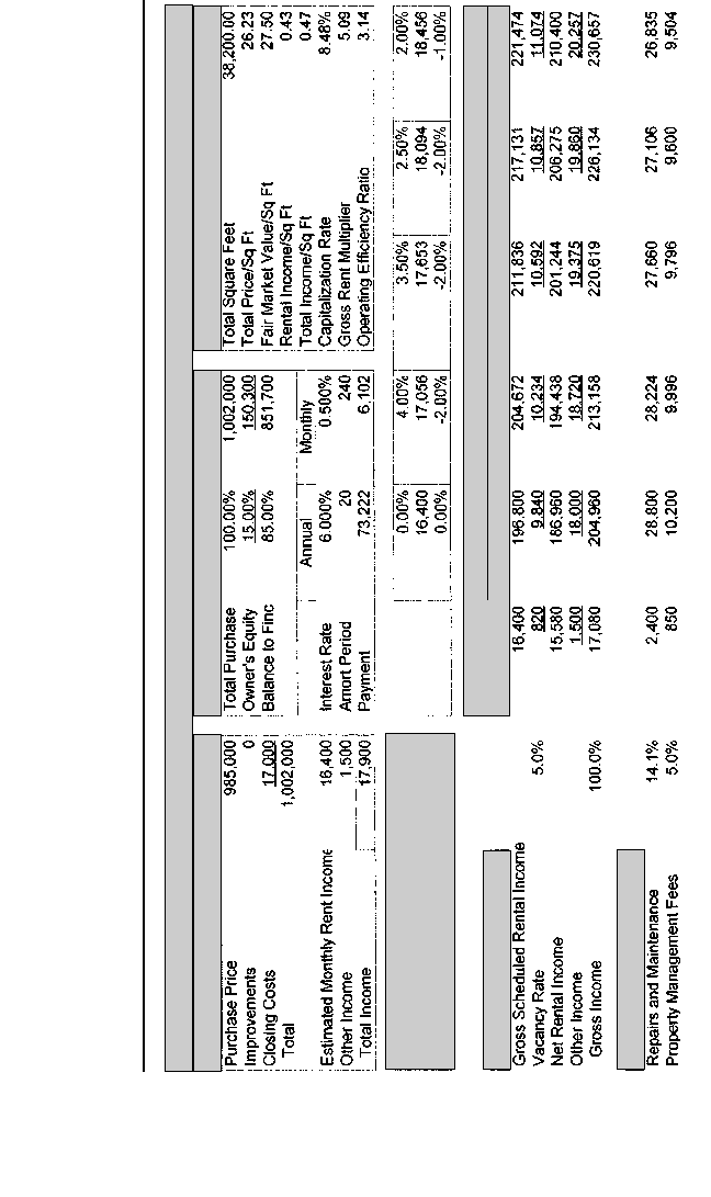
■
94
■
Table 6.2 Debt Service Coverage Ratio
Rental Increase Projections
Average Monthly Rent
Operating Expense Projections
Operating Revenues
Operating Expenses
Actual Projected
Monthly Year 1 Year 2 Year 3 Year 4 Year 5
Cost and Revenue Assumptions
Key Rent RatiosFinancing Assumptions
Financing and Income Analysis
11532_Berges_c06.k.qxd 7/6/04 11:37 AM Page 94
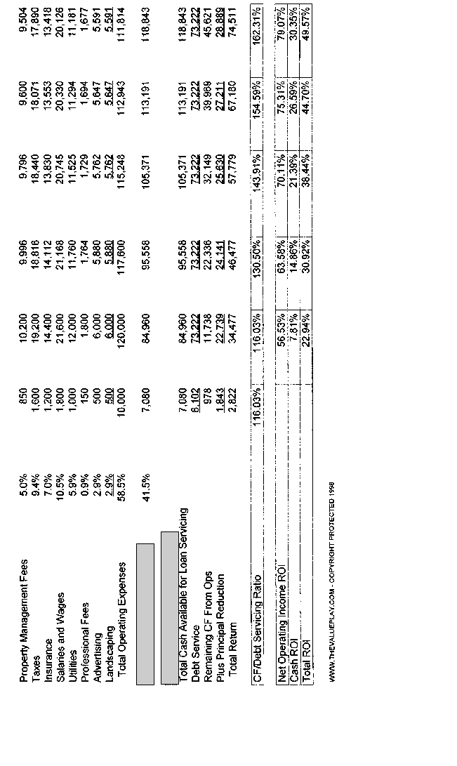
■
95
■
Net Operating Income
Cash Flow From Operations
11532_Berges_c06.k.qxd 7/6/04 11:37 AM Page 95
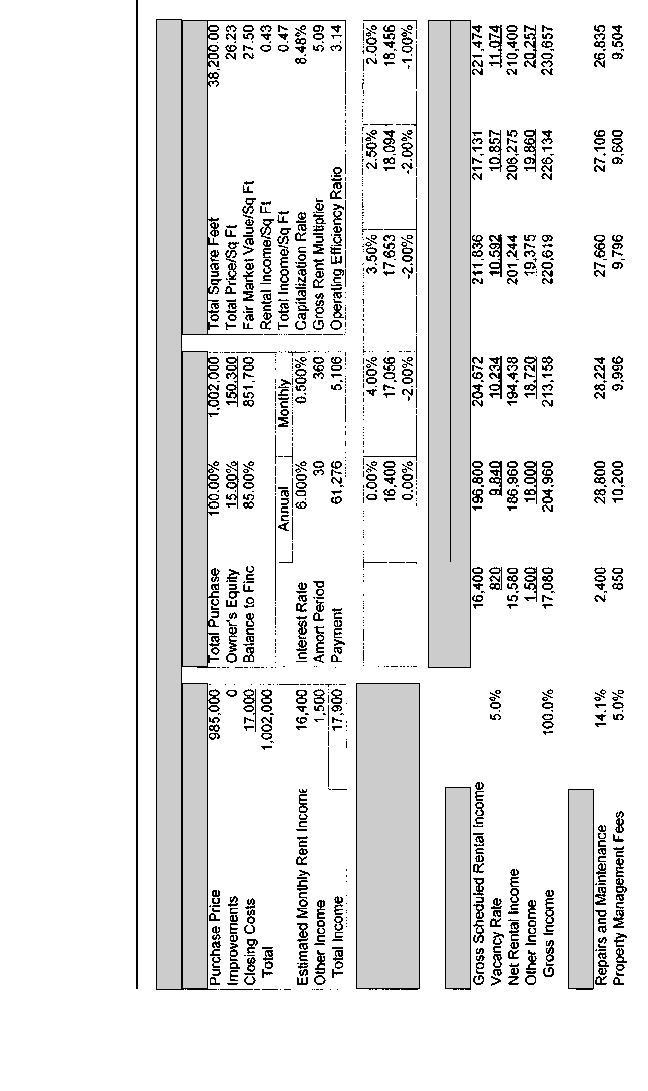
■
96
■
Table 6.3 Debt Service Coverage Ratio
Rental Increase Projections
Average Monthly Rent
Operating Expense Projections
Operating Revenues
Operating Expenses
Actual Projected
Monthly Year 1 Year 2 Year 3 Year 4 Year 5
Key Rent Ratios
Cost and Revenue Assumptions
Financing Assumptions
Financing and Income Analysis
11532_Berges_c06.k.qxd 7/6/04 11:37 AM Page 96
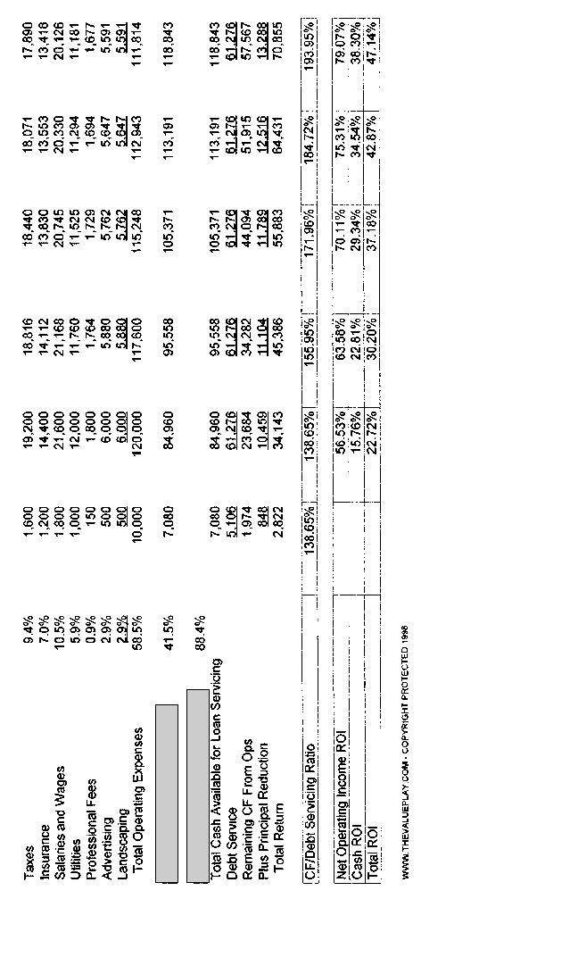
■
97
■
Net Operating Income
Cash Flow From Operations
11532_Berges_c06.k.qxd 7/6/04 11:37 AM Page 97

the relationship between operating expenses and size and can there-
fore be a useful measurement in evaluating similar properties. If the
average OER in a specific market is 3.00, or $3.00 per square foot,
then this property would be considered to be within range, but
slightly above average.
GROSS RENT MULTIPLIER
The next performance measurement is referred to as the gross rent
multiplier (GRM). The gross rent multiplier measures the relation-
ship between the total purchase price of a property and its gross
scheduled income. It is the ratio of price to income. The GRM cal-
culation is made as follows:
Gross rent multiplier ==GRM
The GRM is similar to the cap rate in that it captures the relation-
ship between revenues and price; however, there are two primary
differences. The first is that while the GRM measures the relation-
ship between gross revenues and price, the cap rate measures the
relationship between net revenues, or NOI, and price. The second
difference is that one ratio is inverted compared to the other. For
example, purchase price is the numerator in the GRM quotient, but
it’s the denominator in the cap rate. While a higher cap rate is pre-
ferred to a lower cap rate, a lower GRM is preferred to a higher
GRM. This is true because the ratio will decrease the lower the pur-
chase price is relative to income. It will also decrease the higher the
income is relative to the purchase price.
In the examples illustrated in Tables 6.2 and 6.3, the GRM of 5.09
measures the relationship between the total purchase price and the
gross scheduled income in Year 1.
GRM ==5.09
$1,002,000
ᎏᎏ
$196,800
purchase price
ᎏᎏᎏ
gross scheduled income
■
Real Estate Finance for Investment Properties
■
■
98
■
11532_Berges_c06.k.qxd 7/6/04 11:37 AM Page 98

In the model used to make the calculation, both improvements
and closing costs have been factored into the analysis. Although
there are no improvements in this example, they are typically
included if major capital expenditures are expected. If the
improvements are expected to increase the gross revenues, that,
too, should be taken into consideration. The GRM can be cal-
culated on either an as-is basis with no changes or improvements
to the property, or on a pro forma basis, which includes both
improvements and the expected increase in revenues that would
result from the improvements.
OPERATING RATIO
The next performance measurement used to analyze income pro-
ducing properties is the operating ratio (OR), which is the ratio
between total operating expenses and gross income. Like the oper-
ating efficiency ratio, it provides a gauge of how efficiently a given
property is being operated. Whereas the OER measures efficiency
relative to a property’s total square footage, the OR measures effi-
ciency relative to a property’s income. The calculation is made as
follows:
Operating ratio ==OR
Depending on the type of income property, an OR can range from
about 30 percent to as high as 70 percent or even more. Commercial
properties tend to have a lower OR since most of the expenses are
passed through to the tenant. Multifamily properties, on the other
hand, tend to have a somewhat higher OR since the expenses that are
passed through vary. For example, an apartment building being
operated as an “all bills paid” property will certainly have higher
expenses relative to its income compared to a similar property in
which the utilities are paid by the tenants.
In the examples illustrated in Tables 6.2 and 6.3, the OR of
total operating expenses
ᎏᎏᎏ
gross income
■
Real Estate Investment Performance Measurements and Ratios
■
■
99
■
11532_Berges_c06.k.qxd 7/6/04 11:37 AM Page 99

58.5 percent measures the relationship between total operating
expenses and gross income and is calculated as follows:
OR ==58.5%
The result in this example of 58.5 percent is somewhat on the high
side, but does not fall outside the range of normal ratios. An investor
looking to create value in an income-producing property would
carefully examine each factor that contributes to the operating
expenses. In other words, a high OR may signal that repairs and
maintenance are abnormally high, or perhaps that management
expenses could be trimmed. Conversely, an unusually low OR could
signal that not all of the operating expenses are being reported. If
repairs and maintenance, for example, are known to average 10 to
15 percent of gross income but are being reported as only 3 or 4 per-
cent, then either the property is in exceptionally good condition or
not everything is being reported.
BREAK-EVEN RATIO
The final investment performance measure we examine is known as
the break-even ratio (BER), which measures the relationship
between total cash inflows and total cash outflows. The BER is sim-
ilar to the OR in that both ratios use total operating expenses as part
or all of the numerator and gross income as the denominator. The
difference between the two is that the BER includes as part of the
numerator the debt service. The BER serves as a performance meas-
urement of cash flows from a property, and the OR serves as a per-
formance measurement of income and expenses.
As the break-even ratio’s name implies, the break-even point is
the point at which the total cash inflows are exactly equal to the total
cash outflows. A property with a negative cash flow has a ratio
greater than 1.0, which means that its cash outflows exceed its cash
inflows; conversely, a property with a positive cash flow has a ratio
$120,000
ᎏ
$204,960
■
Real Estate Finance for Investment Properties
■
■
100
■
11532_Berges_c06.k.qxd 7/6/04 11:37 AM Page 100

less than 1.0, which means that its cash inflows exceed its cash out-
flows. The break-even ratio is calculated as follows:
Break-even ratio =
= BER
In the examples illustrated in Tables 6.2 and 6.3, the BER would be
calculated by adding the total operating expenses of $120,000 to the
debt service of $61,276 and then dividing this sum by the property’s
gross income of $204,960. Take a moment to review the calculation.
BER ==88.4%
The property in this example has a positive cash flow since
the BER is 88.4 percent, which is less than 1.0, or 100 percent. I
strongly recommend to investors who have adopted a buy-and-hold
strategy to invest in only those properties that have a positive cash
flow and a BER of less than 1.0. To do otherwise means that addi-
tional cash must be invested each month. A property with a negative
cash flow is just like my three growing sons. They are constantly
hungry and have to be fed all the time! Unless you have deep pock-
ets, a hungry property will eat your lunch if you’re not careful! If
you’re buying a property for the purpose of a quick rehab or flip,
then a positive cash flow isn’t as important, because you don’t need
as much cash to sustain the project. The negative cash flow, along
with the building improvements, is factored into the analysis to
determine whether the project represents a viable opportunity.
In summary, each of the 10 real estate investment performance
measurements discussed in this chapter can be used by investors to
assist in properly analyzing potential investment opportunities. Wise
investors who elect to master these principles will no doubt gain
greater insight into property values and their worth relative to alter-
native opportunities.
$120,000 + $61,276
ᎏᎏᎏ
$204,960
total operating expenses + debt service
ᎏᎏᎏᎏ
gross income
■
Real Estate Investment Performance Measurements and Ratios
■
■
101
■
11532_Berges_c06.k.qxd 7/6/04 11:37 AM Page 101

11532_Berges_c06.k.qxd 7/6/04 11:37 AM Page 102

Chapter 7
Advanced Real Estate
Investment Analysis
In the previous chapter, we examined 10 different real estate invest-
ment performance measurements, which enabled us to better under-
stand how an income-producing property was performing at a given
point in time. These measurements are considered to be static mea-
surements, meaning that they do not take into account a property’s
performance over more than one time period. Instead, performance
is measured at either a specific point in time or over one period of
time, for example, one month or one year. This chapter focuses on
advanced methods of real estate investment analysis by measuring
performance over multiple periods of time. These financial concepts
deal with the time value of money and are especially helpful to indi-
viduals investing in real estate over a prolonged period of time.
FUTURE VALUE ANALYSIS
The first of these financial measurements is referred to as future
value (FV). The future value concept seeks to determine the value of
an investment over multiple periods of time by using the principle of
compounding. This principle is used to attribute the interest earned
on interest. For example, interest as it applies to money is simply the
cost of money to the borrower and the income to the lender. Com-
pound interest is the interest paid on the interest to the borrower and
■
103
■
11532_Berges_c07.k.qxd 7/6/04 11:38 AM Page 103

the interest earned on the interest by the lender. The future value
concept helps investors to know what a particular property will be
worth over a given period of time.
Let’s look at a simple example to better understand the concept of
future value and compounding. Banker Smith has offered to pay
Investor Jones 5 percent annually for a certificate of deposit held for
three years. How much will Investor Jones’s initial investment of
$1,000 be worth at the end of the three-year period? To find the solu-
tion, we start by introducing the following terms.
PV = present value = the value of an investment today
FV = future value = the value of an investment at some point in
the future
i = the interest rate
n = the number of periods
In this example, our terms are applied as follows:
PV = $1,000
FV = ?
i = 5.00%
n = 3 years
FV in Year 1 = $1,000.00 (1 + .05) = $1,000.00 × 1.05 = $1,050.00
FV in Year 2 = $1,050.00 (1 + .05) = $1,050.00 × 1.05 = $1,102.50
FV in Year 3 = $1,102.50 (1 + .05) = $1,102.50 × 1.05 = $1,157.63
In this example, at the end of Year 3, Investor Jones would receive a
total of $1,157.63 from Banker Smith. Now let’s look at solving the
same problem another way.
FV = PV (1 + i)
3
FV = $1,000 (1 + .05)
3
FV = $1,000 (1.1576)
FV = $1,157.63
Applying future value principles to real estate helps investors
determine the value of their invested capital at some distant point in
■
Real Estate Finance for Investment Properties
■
■
104
■
11532_Berges_c07.k.qxd 7/6/04 11:38 AM Page 104

the future. A working knowledge of the principle of compounding is
essential to understanding the effects of returns which are generated
over multiple periods of time. It is this compounding component
that allows the growth of an investment to accelerate over time. Take
a moment to review Exhibit 7.1.
Exhibit 7.1 illustrates the difference between growth rates in an
initial investment of $1,000 earning 10 percent per year over a 25-
year period. The line that curves up sharply is earning interest at a
compounded rate, and the line that is linear is earning interest at a
simple rate. The future value of a $1,000 investment earning 10 per-
cent interest and compounded annually over 25 years is $9,850. By
comparison, the future value of a $1,000 investment earning 10 per-
cent simple interest annually over 25 years is only $3,400. In this
example, the power of compounding has allowed one investment to
grow at a rate almost three times faster than the other investment.
■
Advanced Real Estate Investment Analysis
■
■
105
■
$10
$8
$6
$4
$2
$0
Thousands
25-year period
Compound Interest
Simple Interest
Exhibit 7.1
Effect of compound interest versus simple interest.
11532_Berges_c07.k.qxd 7/6/04 11:38 AM Page 105

Now take a moment to study Table 7.1. This table provides the
factor or value by which an investment can be multiplied to calculate
its future value at a specific interest rate and time period. For exam-
ple, to find out how much a $25,000 investment growing at a rate of
12 percent would be worth in 15 years, locate the corresponding
value in the table and multiply it by the amount of the investment, as
follows:
FV of $25,000 at 12% in 15 years, where
PV = $25,000
i = 12.00%
n = 15 years
Corresponding value from Table 7.1 = 5.47357
FV = $25,000 × 5.47357 = $136,839
Although Table 7.1 is useful in helping to determine the future
value of an investment, it is limited to the rates and time periods
within the table. A financial calculator, on the other hand, can be
used to calculate the future value of an investment of any size at any
rate over any period of time. Most financial calculators are very easy
to use. As long as any three of the four variables are known, the
fourth one can easily be solved for. As an example, an investor with
$5,000 wants to know how long she must hold an investment grow-
ing at an annual rate of 8 percent before her investment is worth
$25,000. In this example, we must solve for n by entering into the
calculator the known values as follows:
PV = $5,000
FV = $25,000
i = 8.00%
Once these values have been entered, then simply solve for n.
n = 21 years
In summary, the concept of future value enables businesses and
individuals to determine the value of an investment at some point in
■
Real Estate Finance for Investment Properties
■
■
106
■
11532_Berges_c07.k.qxd 7/6/04 11:38 AM Page 106

■
107
■
Table 7.1 Value of $1 at Various Compound Interest Rates and Time Periods
Year 2.00% 4.00% 6.00% 8.00% 10.00% 12.00% 14.00% 16.00% 18.00% 20.00%
1 1.02000 1.04000 1.06000 1.08000 1.10000 1.12000 1.14000 1.16000 1.18000 1.20000
2 1.04040 1.08160 1.12360 1.16640 1.21000 1.25440 1.29960 1.34560 1.39240 1.44000
3 1.06121 1.12486 1.19102 1.25971 1.33100 1.40493 1.48154 1.56090 1.64303 1.72800
4 1.08243 1.16986 1.26248 1.36049 1.46410 1.57352 1.68896 1.81064 1.93878 2.07360
5 1.10408 1.21665 1.33823 1.46933 1.61051 1.76234 1.92541 2.10034 2.28776 2.48832
6 1.12616 1.26532 1.41852 1.58687 1.77156 1.97382 2.19497 2.43640 2.69955 2.98598
7 1.14869 1.31593 1.50363 1.71382 1.94872 2.21068 2.50227 2.82622 3.18547 3.58318
8 1.17166 1.36857 1.59385 1.85093 2.14359 2.47596 2.85259 3.27841 3.75886 4.29982
9 1.19509 1.42331 1.68948 1.99900 2.35795 2.77308 3.25195 3.80296 4.43545 5.15978
10 1.21899 1.48024 1.79085 2.15892 2.59374 3.10585 3.70722 4.41144 5.23384 6.19174
11 1.24337 1.53945 1.89830 2.33164 2.85312 3.47855 4.22623 5.11726 6.17593 7.43008
12 1.26824 1.60103 2.01220 2.51817 3.13843 3.89598 4.81790 5.93603 7.28759 8.91610
13 1.29361 1.66507 2.13293 2.71962 3.45227 4.36349 5.49241 6.88579 8.59936 10.69932
14 1.31948 1.73168 2.26090 2.93719 3.79750 4.88711 6.26135 7.98752 10.14724 12.83918
15 1.34587 1.80094 2.39656 3.17217 4.17725 5.47357 7.13794 9.26552 11.97375 15.40702
16 1.37279 1.87298 2.54035 3.42594 4.59497 6.13039 8.13725 10.74800 14.12902 18.48843
17 1.40024 1.94790 2.69277 3.70002 5.05447 6.86604 9.27646 12.46768 16.67225 22.18611
18 1.42825 2.02582 2.85434 3.99602 5.55992 7.68997 10.57517 14.46251 19.67325 26.62333
19 1.45681 2.10685 3.02560 4.31570 6.11591 8.61276 12.05569 16.77652 23.21444 31.94800
20 1.48595 2.19112 3.20714 4.66096 6.72750 9.64629 13.74349 19.46076 27.39303 38.33760
21 1.51567 2.27877 3.39956 5.03383 7.40025 10.80385 15.66758 22.57448 32.32378 46.00512
22 1.54598 2.36992 3.60354 5.43654 8.14027 12.10031 17.86104 26.18640 38.14206 55.20614
23 1.57690 2.46472 3.81975 5.87146 8.95430 13.55235 20.36158 30.37622 45.00763 66.24737
24 1.60844 2.56330 4.04893 6.34118 9.84973 15.17863 23.21221 35.23642 53.10901 79.49685
25 1.64061 2.66584 4.29187 6.84848 10.83471 17.00006 26.46192 40.87424 62.66863 95.39622
11532_Berges_c07.k.qxd 7/6/04 11:38 AM Page 107

the future by applying the principle of compounding to the amount
of the initial investment. As long as any three of the four variables
are known, the fourth unknown variable can be easily solved for.
PRESENT VALUE ANALYSIS
In the previous section, we examined the concept that deals with the
time value of money as it applies to some point in the future. This
concept, referred to as future value, allows us to determine the worth
of an investment or financial instrument at a future time by intro-
ducing the notion of compounding. In this section, we examine the
exact opposite concept, known as present value (PV). Present value
is derived by adjusting the known future value of an asset at a pre-
determined interest rate, or discount rate, from a known future point
in time backward to its value today. Present value analysis is a tool
used by investment professionals every day in a myriad of business
decisions, including investing in assets such as equipment to be used
for expansion, financial instruments yielding a particular income
stream, and income-producing real estate such as office buildings.
The notion of present value allows investors to calculate the
known future value of an asset or financial instrument in today’s dol-
lars through a process referred to as discounting. For example, it
answers a question such as, “How much do I need to invest today if I
want to retire in 10 years with $1 million in an investment known to
yield 12 percent?” In this example, our terms are applied as follows.
PV = ?
FV = $1,000,000
i = 12.00%
n = 10 years
To solve this problem, recall the future value equation as follows:
FV = PV (1 + i)
n
Now let’s rewrite the equation to solve for the present value of an
asset, as follows:
■
Real Estate Finance for Investment Properties
■
■
108
■
11532_Berges_c07.k.qxd 7/6/04 11:38 AM Page 108

FV = PV (1 + i)
n
PV = FV 1\(1 + i)
n
PV = $1,000,000 1\(1 + .12)
10
PV = $1,000,000 1\(3.1058)
PV = $1,000,000 × .321973
PV = $321,973
You would need $321,973 to invest today in an asset yielding 12
percent to be able to retire in 10 years with $1 million. By experi-
menting with the time and interest rate elements of this equation,
investors can explore various options that may be available to
them. For example, if you don’t have $321,973 today to invest, but
you still want to retire with $1 million, you could either extend the
value of time or increase the yield. Adjusting either one of these
variables would decrease the amount of money needed to achieve
your goal.
Now take a moment to review Table 7.2. This table provides the
factor or value by which an investment can by multiplied to calcu-
late its present value at a specific interest rate and time period. For
example, to calculate the present value of an investment discounted
at a rate of 12 percent that would be worth $25,000 in 15 years,
locate the corresponding value in the table and multiply it by the
amount of its future value, as follows:
PV of $25,000 at 12% in 15 years, where
FV = $25,000
i = 12.00%
n = 15 years
Corresponding value from Table 7.2 = .18270
PV = $25,000 × .18270 = $4,567
The concept of present value calculations is a fundamental and
essential tool used by firms in many aspects of operating their busi-
nesses. While future value calculations rely on the process of com-
pounding to derive value, present value calculations rely on the
process of discounting to derive value. Present value calculations
allow investors to determine the worth of an asset whose future
■
Advanced Real Estate Investment Analysis
■
■
109
■
11532_Berges_c07.k.qxd 7/6/04 11:38 AM Page 109

■
110
■
Table 7.2 Present Value of $1 at Various Compound Interest Rates and Time Periods
Year 2.00% 4.00% 6.00% 8.00% 10.00% 12.00% 14.00% 16.00% 18.00% 20.00%
1 0.98039 0.96154 0.94340 0.92593 0.90909 0.89286 0.87719 0.86207 0.84746 0.83333
2 0.96117 0.92456 0.89000 0.85734 0.82645 0.79719 0.76947 0.74316 0.71818 0.69444
3 0.94232 0.88900 0.83962 0.79383 0.75131 0.71178 0.67497 0.64066 0.60863 0.57870
4 0.92385 0.85480 0.79209 0.73503 0.68301 0.63552 0.59208 0.55229 0.51579 0.48225
5 0.90573 0.82193 0.74726 0.68058 0.62092 0.56743 0.51937 0.47611 0.43711 0.40188
6 0.88797 0.79031 0.70496 0.63017 0.56447 0.50663 0.45559 0.41044 0.37043 0.33490
7 0.87056 0.75992 0.66506 0.58349 0.51316 0.45235 0.39964 0.35383 0.31393 0.27908
8 0.85349 0.73069 0.62741 0.54027 0.46651 0.40388 0.35056 0.30503 0.26604 0.23257
9 0.83676 0.70259 0.59190 0.50025 0.42410 0.36061 0.30751 0.26295 0.22546 0.19381
10 0.82035 0.67556 0.55839 0.46319 0.38554 0.32197 0.26974 0.22668 0.19106 0.16151
11 0.80426 0.64958 0.52679 0.42888 0.35049 0.28748 0.23662 0.19542 0.16192 0.13459
12 0.78849 0.62460 0.49697 0.39711 0.31863 0.25668 0.20756 0.16846 0.13722 0.11216
13 0.77303 0.60057 0.46884 0.36770 0.28966 0.22917 0.18207 0.14523 0.11629 0.09346
14 0.75788 0.57748 0.44230 0.34046 0.26333 0.20462 0.15971 0.12520 0.09855 0.07789
15 0.74301 0.55526 0.41727 0.31524 0.23939 0.18270 0.14010 0.10793 0.08352 0.06491
16 0.72845 0.53391 0.39365 0.29189 0.21763 0.16312 0.12289 0.09304 0.07078 0.05409
17 0.71416 0.51337 0.37136 0.27027 0.19784 0.14564 0.10780 0.08021 0.05998 0.04507
18 0.70016 0.49363 0.35034 0.25025 0.17986 0.13004 0.09456 0.06914 0.05083 0.03756
19 0.68643 0.47464 0.33051 0.23171 0.16351 0.11611 0.08295 0.05961 0.04308 0.03130
20 0.67297 0.45639 0.31180 0.21455 0.14864 0.10367 0.07276 0.05139 0.03651 0.02608
21 0.65978 0.43883 0.29416 0.19866 0.13513 0.09256 0.06383 0.04430 0.03094 0.02174
22 0.64684 0.42196 0.27751 0.18394 0.12285 0.08264 0.05599 0.03819 0.02622 0.01811
23 0.63416 0.40573 0.26180 0.17032 0.11168 0.07379 0.04911 0.03292 0.02222 0.01509
24 0.62172 0.39012 0.24698 0.15770 0.10153 0.06588 0.04308 0.02838 0.01883 0.01258
25 0.60953 0.37512 0.23300 0.14602 0.09230 0.05882 0.03779 0.02447 0.01596 0.01048
11532_Berges_c07.k.qxd 7/6/04 11:38 AM Page 110

value is known in today’s dollars by discounting it back at a speci-
fied or required rate. Understanding the principle of present value
enables business owners to make prudent decisions relating to the
use of available capital for investment purposes.
NET PRESENT VALUE ANALYSIS
In the previous section, we learned about using present value for-
mulas to determine the value of an asset in today’s dollars of a
known future value at a specific discount rate and period of time. In
this section, we examine another financial tool used to measure
investments. It’s known as net present value (NPV). The financial
analysis of assets using net present value calculations is identical to
that of present value calculations with one exception. In a present
value calculation, an investor simply wants to determine how much
should be invested today to earn a particular rate of return over a
given period of time, so solving for PV is all that is required. In a net
present value calculation, however, the cost of the investment is
already known. Because of this, investors seeking to purchase an
income-producing asset use the PV formula to discount the value of
the asset back at a predetermined minimum expected rate of return.
If the present value of the asset exceeds its cost, the difference is a
positive NPV. In this case, the investor would approve the purchase
of the asset since it met or exceeded her minimum expected rate of
return. If, however, the present value of the asset is less than its cost,
the difference results in a negative NPV in which case, the investor
would reject the purchase since it did not meet her minimum
expected rate of return.
Let’s look at an example to better understand how the net present
value calculation can be useful to a business. Assume a business that
has a minimum required rate of return of 8 percent is considering the
purchase of an income-producing asset with a purchase price of
$500,000. The future value of the asset in eight years is expected to
be $1.1 million. Using the minimum required rate of return of 8 per-
cent, should the company purchase the asset? To answer that ques-
tion, we must first solve for its present value.
■
Advanced Real Estate Investment Analysis
■
■
111
■
11532_Berges_c07.k.qxd 7/6/04 11:38 AM Page 111

PV of $1.1 million at 8% in 10 years, where
FV = $1,100,000
i = 8.00%
n = 10 years
Corresponding value from Table 7.2 = .46319
PV = $1,100,000 × .46319 = $509,512
To determine the net present value of this investment, the initial cost
of the asset must now be subtracted from the present value.
NPV = PV − cost
NPV = $509,512 − $500,000 = $9,512
NPV = $9,512
Since the NPV is positive, it meets the minimum rate of return
required by the business and therefore merits further consideration.
A NPV greater than zero means that not only does the asset meet the
minimum rate of return, but by definition, it actually exceeds it. By
substituting the actual cost of the asset for PV, we can solve for i
using a financial calculator, as follows:
PV = $500,000
FV = $1,100,000
n = 10 years
i = ?
Using a financial calculator, enter the values as illustrated for each
of the three known variables. Be sure to enter the PV of $500,000 as
a negative value since it represents a cash flow out. All other vari-
ables should be entered as positive values. The solution for i is as
follows:
PV = $500,000
FV = $1,100,000
n = 10 years
i = 8.20%
■
Real Estate Finance for Investment Properties
■
■
112
■
11532_Berges_c07.k.qxd 7/6/04 11:38 AM Page 112

To summarize, the yield on this investment is 8.20 percent, which
exceeds the minimum rate of return required by the business. When
analyzing these types of investment opportunities, recall that firms
must take into consideration their cost of capital. In this example, if
the company’s cost of capital was 6.00 percent, investing in the asset
would yield an incremental 2.20 percent. The net present value cal-
culation is a tool commonly used by investors from many different
industries, including real estate.
INTERNAL RATE OF RETURN
In the previous section, the financial analysis principle of net
present value enabled us to first calculate the present value of an
investment and then subtract the actual cost of the asset from its
present value. The NPV calculations were made with a minimum
rate of return already established by the firm. In this section, in-
stead of solving for the NPV, we solve for the internal rate of
return (IRR). The IRR calculation measures the yield or rate of
return on an investment rather than its present value. The present
value is assumed to be the initial cost of the asset. The IRR calcu-
lation measures the yield from a series of cash flows across a spec-
ified period of time and includes the cost of the asset, the cash
flows from the asset, and the salvage value of the asset at the end
of its useful life. In the case of plant and equipment, an asset’s use-
ful life may be exhausted at the end of a period due to functional
or technical obsolescence. The useful life of real estate, which may
actually increase in value over time, is said to be exhausted when
the property is divested.
Let’s look at an example. Assume Investor Lincoln wants to add
an additional space to a small retail strip center. Construction costs
to add the space are estimated to be $100,000. As illustrated in
Table 7.3, Lincoln has two choices. In Scenario 1, he can lease the
space to Tenant A on a lease-option agreement for three years at a
rate of $10,000 per year and then sell the space at the end of the
three-year period for $110,000. In Scenario 2, he can lease the
■
Advanced Real Estate Investment Analysis
■
■
113
■
11532_Berges_c07.k.qxd 7/6/04 11:38 AM Page 113

space to Tenant B on a lease option agreement for six years at a
rate of $10,000 per year for the first three years and $12,500 for
the next three years, then sell the space at the end of the six-year
period for $120,000.
The internal rate of return in Scenario 1 is 12.94 percent. The
income generated from three years’ worth of cash flows is the equiv-
alent of earning an annualized rate of return of 12.94 percent on
Investor Lincoln’s initial investment of $100,000. If, however,
Investor Lincoln chooses to hold the property for six years, his yield
increases to 13.40 percent. Because the IRRs in this example are
marginally close, there may be other factors such as tax issues that
could affect Lincoln’s decision to choose one scenario over the
other; however, with all other things being equal, the higher yield in
Scenario 2 suggests that Investor Lincoln should choose this alter-
native over Scenario 1.
Let’s look at another example using The Value Play Income Ana-
lyzer, a proprietary model used for analyzing income properties
such as apartment buildings. In Table 7.4, the cash flows of a 50-unit
apartment building are examined to determine its respective internal
rate of return.
In Table 7.4, note the net cash flows from investment section in
the lower portion of the table. This section is used to display the net
cash flows from the property. The first value in the Year 1 exit sec-
tion of −$514,250 is a cash-flow-out value that represents the
owner’s initial equity. This is followed by a cash-flow-in value of
$683,618, derived by adding the following values.
■
Real Estate Finance for Investment Properties
■
■
114
■
Table 7.3 Internal Rate of Return
Cash Flows Scenario 1 Scenario 2
Initial Investment (100,000) (100,000)
Cash Flow in Year 1 10,000 10,000
Cash Flow in Year 2 10,000 10,000
Cash Flow in Year 3 120,000 10,000
Cash Flow in Year 4 12,500
Cash Flow in Year 5 12,500
Cash Flow in Year 6 132,500
Internal Rate of Return 12.94% 13.40%
11532_Berges_c07.k.qxd 7/6/04 11:38 AM Page 114

Owner’s equity $514,250
After-tax cash flows $97,983
Principal reduction $46,385
Gain on sale $25,000
Total $683,618
The cash flow in value of $683,618 assumes the owner sells the
property at the end of Year 1 at a cap rate of 9.43 percent, which is
comparable to the 9.50 cap rate at the time of purchase (shown in the
key ratios section). If the property was sold at the end of the first
year, based on its projected cash flows it would earn an internal rate
of return of 32.93 percent. Take a moment to review the net cash
flows from investment in Year 3. The initial cash flow out, which is
the owner’s equity, of $514,250 is the same as in the Year 1 scenario.
The income earned from Years 1, 2, and 3 is then factored in, as well
as the reduction in principal and gain on sale of $450,000. Based
on the projected cash flows in the Year 3 scenario, the property
would generate an IRR of 46.05 percent. Now take a moment to
examine the net cash flows from investment in Year 5. The cash
flows are derived in the same manner as in the previous two sce-
narios, but include income and principal reduction for Years 4
and 5 as well. Based on the projected cash flows in the Year 5 sce-
nario, the property would earn an internal rate of return of 40.21
percent.
While the internal rate of return calculation is widely used by
investors to measure the yield on a series of cash flows, there is
one caveat. The IRR calculation works best when the initial cash
flow is negative and all subsequent cash flows are positive. Addi-
tional negative values in the cash flow stream can potentially
create multiple solutions. In an excerpt taken from Investment
Analysis for Real Estate Decisions (Chicago: Dearborn Trade,
1997, p. 222), authors Greer and Kolbe note that the IRR calcula-
tion can be problematic under certain conditions. The authors
assert the following.
■
Advanced Real Estate Investment Analysis
■
■
115
■
11532_Berges_c07.k.qxd 7/6/04 11:38 AM Page 115
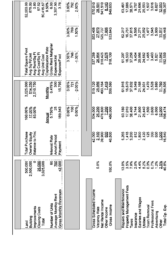
■
116
■
Table 7.4 Property Analysis Worksheet
The Value Play Income Analyzer
Cost and Revenue Assumptions
Financing Assumptions
Key Ratios
Rental Increase Projections
Average Monthly Rent
Operating Expense Projections
Operating Revenues
Operating Expenses
Actual Projected
Monthly Year 1 Year 2 Year 3 Year 4 Year 5
11532_Berges_c07.k.qxd 7/6/04 11:38 AM Page 116
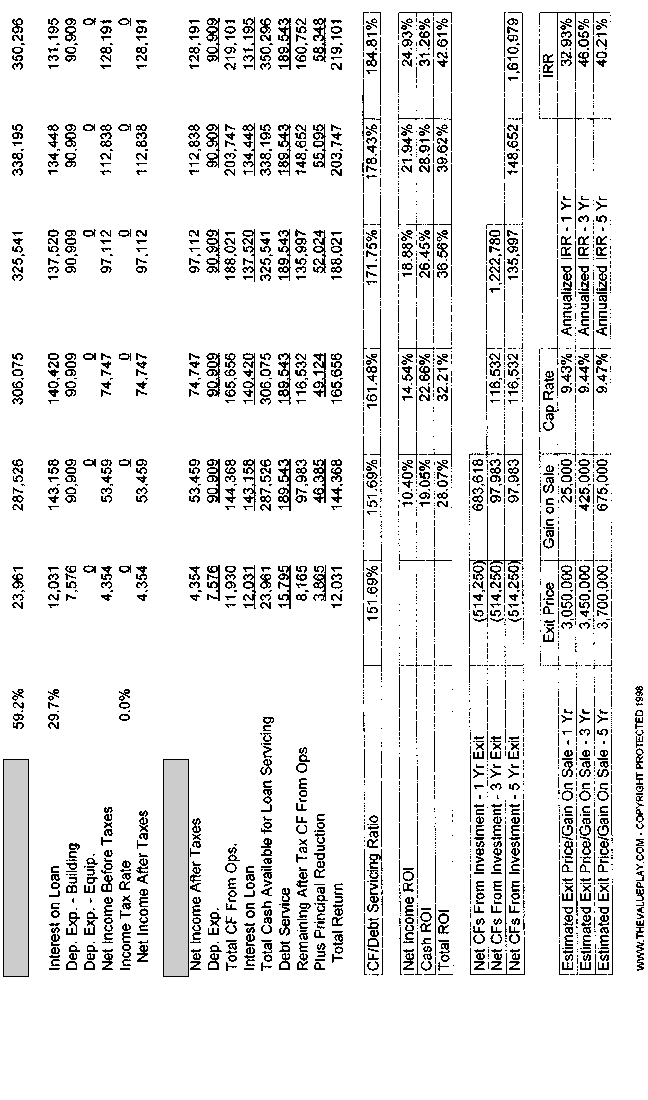
■
117
■
Net Operating Income
Cash Flow From Operations
11532_Berges_c07.k.qxd 7/6/04 11:38 AM Page 117

Problems associated with the internal rate of return can
result in conflicting decision signals from this and other
discounted cash flow approaches. Generally, such a con-
flict arises because the internal rate of return signal is dis-
torted. If heeded, it might result in serious investment error.
Potential dissonance stems from peculiarities of the inter-
nal rate of return equation, which can yield more than one
solution, and from problems associated with the reinvest-
ment assumption inherent in choices among alternative
investments that exhibit different patterns of anticipated
after tax cash flows.
Mathematicians and analysts alike have attempted to resolve the
problems that occur with IRR calculations resulting from the rever-
sal in signals in a series of cash flows. Three of the more common
methods used to address these issues are (1) the modified internal
rate of return, or MIRR, (2) the adjusted rate of return, and (3) the
financial management rate of return. According to Greer and Kolbe,
the MIRR method “solves the multiple root problem by discounting
all negative cash flows back to the time at which the investment is
acquired and compounding all positive cash flows forward to the
end of the final year of the holding period.” The modified approach
eliminates the reversal-of-signals problem and provides a unique
solution for a series of cash flows. The adjusted rate of return
method assumes the investor has in essence borrowed funds from
one period and repaid them in another period, again attempting to
deal with positive and negative changes in values. Finally, the finan-
cial management rate of return method, developed by M. Chapman
Findley and Stephen D. Messner, integrates two intermediate rates.
The first, a cost-of-capital rate, is applied to negative that which are
discounted back to the beginning of the investment time period
where t = 0. The second rate is a reinvestment rate and is applied to
positive values that are compounded forward to the end of the
investment time period.
In summary, this chapter has focused on several advanced meth-
ods of real estate investment analysis by measuring performance
over multiple periods of time. These financial analysis tools enable
■
Real Estate Finance for Investment Properties
■
■
118
■
11532_Berges_c07.k.qxd 7/6/04 11:38 AM Page 118

individuals and businesses to evaluate investments extending over
various periods of time and having various streams of cash flow.
Most financial analysis methods use discounting and compounding
calculations to express the sum of a stream of cash flows in either
present value or future value terms, thereby enabling investors to
make decisions based on predetermined minimum rates of return.
■
Advanced Real Estate Investment Analysis
■
■
119
■
11532_Berges_c07.k.qxd 7/6/04 11:38 AM Page 119

11532_Berges_c07.k.qxd 7/6/04 11:38 AM Page 120

Chapter 8
The Valuation of Real Property
APPRAISAL DEFINED
An appraisal is an estimate of an object’s worth or value.
Appraisals are used to determine the value of both personal prop-
erty and real property. For example, you may want to have an inde-
pendent appraisal done on a diamond ring with a $20,000 price tag
before investing that kind of money in it. The appraisal could then
be used for insurance purposes in the event the ring was lost or
stolen. Appraisals are also used to determine the worth and value of
real property, such as land or buildings. In Income Property Valua-
tion (Massachusetts: Heath Lexington Books, 1971, p. 9), author
William N. Kinnard states the following as it relates to the appraisal
process:
An appraisal is a professionally derived conclusion about
the present worth or value of specified rights or interests in
a particular parcel of real estate under stipulated market
conditions or decision standards. Moreover, it is (or should
be) based on the professional judgment and skill of a
trained practitioner. Its conclusions should be presented in
a thoroughly logical and convincing way to a client or an
interested third party who requires the value estimate to
help make a decision or solve a problem involving the real
estate in question.
■
121
■
11532_Berges_c08.k.qxd 7/6/04 11:40 AM Page 121

An appraisal opinion is usually delivered in written
form. A professional appraisal report should contain as a
minimum the essential ingredients of an appraisal identi-
fied as (1) the identity and legal description of the real
estate; (2) the type of value being estimated; (3) the inter-
ests being appraised; (4) the market conditions or decision
standards in terms of which the value estimate is made (fre-
quently identified by specifying an “as of” date or effective
date for the appraisal); and (5) the value estimate itself.
Moreover, the report should indicate the data and reason-
ing employed by the appraiser in reaching his value con-
clusion, any special or limiting conditions that impinged
on his analysis and conclusion, and the appraiser’s certifi-
cation and signature.
THE NATURE OF PRICE AND VALUE
As Kinnard clearly states, the process for appraising real property is
well defined and specific. Although objective in its format, property
values vary widely for many reasons. A 1,000-square-foot house
with three bedrooms and two baths, for example, may be worth only
$60,000 in Dallas, Texas, while in Hollywood, California, that same
house may sell for $150,000. Real estate values are impacted by
many different micro- and macroeconomic forces, including supply
and demand issues, the current interest rate environment, local and
national economic conditions, the desirability of the location, and
differences in tax rates. The same appraisal standards applied to a
particular piece of real property in one region may yield entirely dif-
ferent results for a similar piece of real property in another region.
Likewise, an appraisal of those same properties today would almost
certainly be different than an appraisal conducted 10 years ago.
Although the terms price and value are similar in meaning, they
are not the same. An appraisal is an estimate of value and provides
no indication of what price will actually be paid for a piece of real
property. For example, an individual shopping for a new refrigerator
will first determine all the desired features she must have, and then
begin to shop for one matching her requirements. Once a model is
■
Real Estate Finance for Investment Properties
■
■
122
■
11532_Berges_c08.k.qxd 7/6/04 11:40 AM Page 122

selected, she will then most likely shop around at several locations
to determine which store is offering the best price. By purchasing
the refrigerator at the lowest price available, not only is the buyer
able to save money, but she is also said to have received the best
value. Although two identical refrigerators at two different locations
may have the same resell value, the one that originally sold for less
money has a greater equivalent value.
The appraisal provides the basis for price, but buyers and sellers
are free to negotiate. Kinard asserts, “In the perfect market of eco-
nomic theory, informed and rational buyers would pay no more, and
informed and rational sellers would accept no less, than the present
worth of the anticipated future benefits from ownership of an asset.”
As a result of various differences in economic conditions, however,
the actual price paid may be, and often is, different than the stated
value in an appraisal report. Price is therefore a reflection of the
past. It is what has already occurred. Value, on the other hand,
reflects the price that should be paid “in the perfect market of eco-
nomic theory.” Value is therefore a forecast of price. It is what may
occur at some point in the future, not what has occurred at some
point in the past.
THREE PRIMARY APPRAISAL METHODS
Three primary methods are used by appraisers to determine the
value of real estate: the replacement cost method, the sales compar-
ison method, and the income capitalization method. (See Exhibit
8.1). Each method of valuation has its place and serves a unique
function in assessing the worth of real property. Commercial prop-
erties such as retail centers, office buildings, and apartment com-
plexes, for example, rely primarily on the income method, while
single-family houses typically rely on the sales comparison method.
REPLACEMENT COST METHOD
The replacement cost method, or cost approach, is most commonly
used for estimating the replacement value of physical assets for
■
The Valuation of Real Property
■
■
123
■
11532_Berges_c08.k.qxd 7/6/04 11:40 AM Page 123

insurance purposes. For example, should a house be destroyed in a
hurricane, an insurance company would want to know the actual
cost to replace it. The income method and the sales comparison
method are of little or no consequence in estimating replacement
costs. The insurance policy you have on your personal residence
most likely includes a replacement cost policy with built-in pre-
mium adjustments that automatically increase each year due to rises
in labor and material costs. Butler Burgher, Inc., an appraisal firm in
Houston, Texas, stated the following in an appraisal report that was
completed for one of my apartment projects.
The cost approach is based on the premise that the value of
a property can be indicated by the current cost to construct
a reproduction or replacement for the improvements
minus the amount of depreciation evident in the structures
from all causes plus the value of the land and entrepre-
neurial profit. This approach to value is particularly useful
for appraising new or nearly new improvements.
The replacement cost approach is most commonly used when
estimating the actual costs associated with replacing the physical
assets of a house or building. For example, for an office building
■
Real Estate Finance for Investment Properties
■
■
124
■
Exhibit 8.1
Three primary appraisal methods.
1. Replacement cost method
2. Sales comparison method
3. Income capitalization method
11532_Berges_c08.k.qxd 7/6/04 11:40 AM Page 124

completely destroyed by fire, the value established from the cost
approach would be useful in helping to determine exactly how much
an insurance company would pay for the resulting damages.
An additional factor taken into consideration when the replace-
ment cost approach is used is depreciation, which encompasses
deterioration, functional obsolescence, and external obsolescence.
Deterioration is said to occur when property loses value because
of average wear and tear over a period of time. For example, a 10-
year-old roof that has a 25-year life is said to have deteriorated, or
depreciated, by 10/25, or 40 percent. Functional obsolescence is
described as a loss in property value resulting from outdated home
designs or mechanical equipment. The value of a house with only
gas space heaters rather than central heating, for example, would
be adversely affected. Finally, external obsolescence is described
as a loss in property value resulting from changes in the sur-
rounding neighborhood or community. For instance, the value of a
house would be adversely affected if it were located in a neigh-
borhood that had experienced a significant increase in crime. An
increase in traffic and noise levels may also contribute to a decline
in value.
The underlying rationale of the replacement cost approach is that
an informed buyer would not be willing to pay more for a particular
house than the cost of building an identical house on a comparably
sized lot in a similar neighborhood. The basic formula for calculat-
ing the replacement cost approach is as follows:
Replacement cost = cost of construction − depreciation
+ land value
Let’s look at an example. Assume the subject property is similar
in design, size, and quality to a new house that costs $100,000 to
build, not including the lot. The subject property is 30 years old and
has depreciated in value by 25 percent due to normal wear and tear,
as well as a general decline in the neighborhood in which it is
located. The value of the lot is estimated at $20,000. Using the
replacement cost approach, the value of the subject property is cal-
culated as follows:
■
The Valuation of Real Property
■
■
125
■
11532_Berges_c08.k.qxd 7/6/04 11:40 AM Page 125

Replacement cost = $100,000 − ($100,000 × 25%) + $20,000
Replacement cost = $100,000 − $25,000 + $20,000 = $95,000
In this example, since the subject property has declined in value,
using the replacement cost approach indicates a value of $95,000.
This compares to a total value of $120,000 for a new house, which
includes a comparable lot, for a difference of $25,000, the amount of
loss suffered by the subject property from depreciation.
SALES COMPARISON METHOD
The second primary appraisal method is the sales comparison
method, or market approach, which is the method deemed most
appropriate for the proper determination of value for single-family
houses. This includes both owner-occupied and non-owner-
occupied single-family dwellings. The sales comparison method is
by far the most commonly used approach of the three methods,
because the number of single-family dwellings is much greater than
any other type of property. This method is based on the logic that the
price paid for recent sales of like properties represents the price buy-
ers are willing to pay and is therefore representative of true market
value. The price paid may vary for many reasons, including changes
in interest rates, changes in unemployment rates, changes in general
economic conditions, as well as changes in the cost of materials and
land. All of these factors combine to cause changes in the supply and
demand of available properties.
The sales comparison method is based on the premise of substitu-
tion and maintains that a buyer would not pay more for real property
than the cost of purchasing an equally desirable substitute in its
respective market. This method also assumes that all comparable
sales used in the appraisal process are legitimate arm’s-length trans-
actions to help ensure accuracy of the data used in the report. The
sales comparison method furthermore provides that comparable
sales used have occurred under normal market conditions. For
example, this assumption would exclude properties bought and sold
■
Real Estate Finance for Investment Properties
■
■
126
■
11532_Berges_c08.k.qxd 7/6/04 11:40 AM Page 126

under foreclosure conditions—that is, those purchased from a
bank’s real estate owned, or REO, portfolio.
The sales comparison method typically examines three or more
like properties and adjusts their value based on similarities and dif-
ferences among them. For example, if the subject property had a
two-car garage and the comparable property had a three-car garage,
an adjustment would be made for the difference to bring the values
more in line with each other. In this case, the comparable property’s
value would be adjusted downward to compensate for the additional
garage unit. In other words, the value of the additional garage unit is
subtracted to make it the equivalent of a two-car garage. Butler
Burgher provides further clarification of the sales comparison
method:
The sales comparison approach is founded upon the prin-
ciple of substitution which holds that the cost to acquire an
equally desirable substitute property without undue delay
ordinarily sets the upper limit of value. At any given time,
prices paid for comparable properties are construed by
many to reflect the value of the property appraised. The
validity of a value indication derived by this approach is
heavily dependent upon the availability of data on recent
sales of properties similar in location, size, and utility to
the appraised property.
The sales comparison approach is premised upon the
principle of substitution—a valuation principle that states
that a prudent purchaser would pay no more for real prop-
erty than the cost of acquiring an equally desirable substi-
tute on the open market. The principle of substitution
presumes that the purchasers will consider the alternatives
available to them, that they will act rationally or prudently
on the basis of their information about those alternatives,
and that time is not a significant factor. Substitution may
assume the form of the purchase of an existing property
with the same utility, or of acquiring an investment which
will produce an income stream of the same size with the
same risk as that involved in the property in question. . . .
■
The Valuation of Real Property
■
■
127
■
11532_Berges_c08.k.qxd 7/6/04 11:40 AM Page 127

The actions of typical buyers and sellers are reflected in the
comparison approach.
According to Butler Burgher, the sales comparison appraisal
method examines like properties and adjusts their respective values
based on similarities and differences between them. This method is
most often used in valuing single-family houses. Recall that the
objective of using this method is to determine the subject property’s
value. Unlike the cost approach, which seeks to establish the cost of
reconstruction for the subject property, the sales comparison
approach seeks to establish its market value. Recall also that the
market value of a property is not the same as its price. The
appraiser’s objective is to determine a value that reflects the most
likely price a buyer is willing to pay for a particular property given
similar properties to choose from.
While the use of sales comparables, or comps, as they are also
referred to, is an important factor to consider in the analysis of esti-
mating the value of larger income-producing properties, greater
weight is usually given to the income capitalization method dis-
cussed in the next segment. The sales comparison method is
designed to examine and compare the physical attributes of real
property, not the income generated by it.
INCOME CAPITALIZATION METHOD
The third primary appraisal method is the income capitalization
method, used to value real property that generates some type of
income, which is employed for investment purposes. In Income
Property Valuation, author Kinard describes the process of capital-
ization as follows:
Real estate is a capital good. This means that the benefits
from owning it—whether in the form of money income or
amenities, or both—are received over a prolonged period
of time. Operationally, this means more than one year; in
fact, it is typically for 10, 20, 40 or more years.
■
Real Estate Finance for Investment Properties
■
■
128
■
11532_Berges_c08.k.qxd 7/6/04 11:40 AM Page 128

* * * Free PDF Preview End * * *
Purchase Required To Gain Total Access
!